


请先登录您的atyun账户,方可使用该功能

审核通过后即可使用此功能,请耐心等待~


深度学习:如何理解tensorflow文本含义识别的原理
2017年07月31日 由 xiaoshan.xiang 发表
31833
0
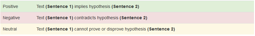
文本含义识别是一个简单的逻辑练习,用来判断一个句子是否可以从另一个句子推断出来。承担了文本含义识别任务的计算机程序,试图将一个有序的句子分类为三个类别中的一种。第一类叫做“positive entailment”,当你用第一个句子来证明第二个句子是正确的时候就会出现。第二个类别是“negative entailment”,是positive entailment的反面。当第一个句子被用来否定第二个句子时,就会出现这种情况。最后,如果这两个句子没有关联,那么它们就被认为是“neutral entailment”。
作为应用程序的一个组成部分,文本含义识别是有用的。例如,问答系统可以使用文本含义识别来验证存储信息的答案。其他自然语言处理系统(NLP)也发现类似的应用。
本文将引导你了解如何构建一个简单快捷的神经网络来执行使用TensorFlow.的文本含义识别。
除了安装 TensorFlow version 1.0之外,还要确保安装:
Jupyter
Numpy
Matplotlib
为了在神经网络训练中获得更多的进步,可以安装 TQDM,但这不是必需的。请访问GitHub上的这篇文章的代码和Jupyter笔记本(链接为https://github.com/Steven-Hewitt/Entailment-with-Tensorflow)。我们将使用斯坦福的SNLI数据集来进行我们的训练,使用Jupyter Notebook中的代码下载并提取我们需要的数据。如果这是你第一次使用TensorFlow,我建议你看看Aaron Schumacher的文章“Hello, Tensorflow”。
将从所有必要的输入开始,利用Jupyter Notebook显示图表和图像。
在本节中,我们将通过一些文本含义识别的例子来说明positive, negative和 neutral entailment。首先,我们来看看positive entailment——例如,当你读到“Maurita and Jade both were at the scene of the car crash”时,你可以推断“Multiple people saw the accident”。在这个例句中,我们可以用第一个句子(也称为“文本”)证明第二句(也称为“假设”),这代表是positive entailment。鉴于莫丽塔和杰德都看到车祸,说明有多人看到。
让我们考虑另一个句子对。“在公园里和老人一起玩的两只狗”推导“那天公园里只有一只狗”。第一句话说有“两只狗”,那么就说明公园至少有两只狗,第二句话与这个观点相矛盾,所以是negative entailment。
最后,为了阐明neutral entailment,我们看“我和孩子们打棒球”和“孩子们爱吃冰淇淋”这两句话,打棒球和爱吃冰淇淋完全没有任何关系。我可以和冰淇淋爱好者打棒球,我也可以和不喜欢冰淇淋的人打棒球(两者都是可能的)。因此,第一句话没有说明第二句话的真实或虚假。
对于神经网络来说,它们主要使用数字值工作。为了解决这个问题,我们需要用数字来表示我们的单词。这些数字意味着什么,例如,我们可以使用字母中的字符代码,但这并没有告诉我们任何关于它的含义(这意味着TensorFlow不得不做大量的工作来说明“dog”和“canine”是接近相同的概念)。将类似的意义转化为神经网络可以理解的过程,这个过程被称为word vectorization。
常用的创建word vectorization的方法是让每个单词表示一个非常高维空间中的一个点。具有相似含义的单词应该在这个空间中相对接近。这一点的演示在 word vectorization的TensorFlow教程中可以找到(链接地址是https://www.tensorflow.org/tutorials/word2vec)。
我们不需要创建一个新的表达形式。如果通用数据不够用,可以用已经存在的一些很好的通用矢量表现形式和训练专业材料的方法。
我们将使用60亿的Wikipedia 2014 + Gigaword 5向量,因为它是最小并且最容易下载的。我们将以编程方式下载该文件,运行它可能需要一段时间(这是一个相当大的文件)。
与此同时,我们收集我们的textual entailment数据集:斯坦福大学SNLI数据集。
现在我们已经下载了GloVe向量,将它们加载到储存器中,将空间分隔的格式反序列化为Python字典:
通过神经网络来处理句子。让我们从制作这个序列开始:
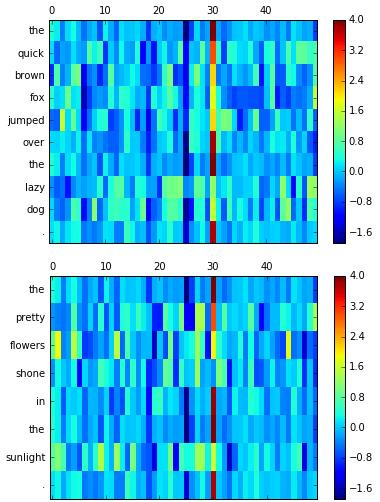
为了更好地理解word vectorization过程以及算机研究句子时所看到的东西,我们可以将这些向量表示为图像。使用notebook 将句子可视化。每一行表示一个词,而列表示word vectorization的个体维度。word vectorization是在根据单词与其他单词的关系进行训练的,实际上表示的含义是含糊不清的。但计算机能理解这种向量语言,这是最重要的部分。一般来说,在相同的位置上颜色相似的两个向量表示单词在意义上相似。
与图像不同的是,句子有固有的顺序,且不受大小的约束,所以我们需要一种新的不完全连接前馈网络的神经网络类型,这是因为前馈网络占据一个输入值并且只需运行到产生一个输出,而我们需要循环。
Recurrent neural networks(RNNs)是神经网络的一种序列学习工具。这种类型的神经网络只有一层的隐藏输入,它被重复用于序列中的每个输入,以及传递给下一个输入计算的“memory”。
对序列中的每一个输入重复同样的计算,这意味着Recurrent neural networks的一个“层”可以被展开成许多层。这使得神经网络能够处理一个非常复杂的句子。TensorFlow有一个简单的RNN cell,BasicRNNCell的实现,它可以添加到你的TensorFlow中,如下图:
从理论上讲,神经网络将能够记住来自第一层的东西,甚至是一个早期句子的结尾。这种循环形式的主要问题是:在实践中,早期的数据被更新的并不重要的输入和信息完全淹没。Recurrent neural networks或者是带有标准隐藏单位的神经网络不能长时间维持信息。这个故障被称为梯度消失问题。
最简单的方法就是通过示例可视化。在最简单的情况下,输入和“memory”权重大致相同。数据的第一个输入将影响第一个输出的大约一半(另一半是启动“memory”),第二次输出的四分之一,然后是第三输出的八分之一,等等。
这意味着我们不能使用vanilla循环网络,如果我们想要对这两个句子进行追踪。解决方案是使用不同类型的循环网络层。也许最简单的就是长短期记忆层,也就是LSTM。
在LSTM中,代替计算当前储存器时每次都使用相同方式的输入(xt),神经网络可以通过“输入门”(it)决定当前值对储存器的影响程度,并做出一个决定;通过被命名为“忘记门”(ft)的遗忘的存储器(ct)做出另外一个决定,根据储存器将哪些部分通过“输出门”(ot)发送到下一个时间步长(ht)做第三个决定。
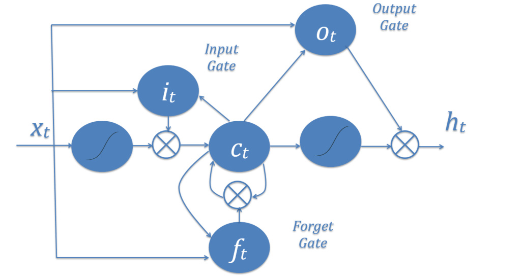
这三个门的组合创造了一个选择:一个单一的LSTM节点,可以将信息保存在长期储存器中,也可以将信息保存在短期储存器中,但不能同时进行。短期记忆LSTMs训练的是相对开放的输入门,让大量的信息进来,也经常忘记很多;而长期记忆LSTMs有紧密的输入门,只允许非常小的,非常具体的信息进入。这种紧密性意味着它不会轻易失去它的信息,并且允许保存更长的时间。
总的来说,LSTMs是非常神秘的。不同LSTM节点在同一个神经网络可能会有彼此依赖但又截然不同的门。
我们不打算在我们的神经网络中使用 vanilla RNN层,所以我们会清除图表并添加一个LSTM层,默认情况下也包含TensorFlow。这将是我们神经网络的第一部分,定义神经网络的需要的所有常数:
我们还将重新设置图表,不包括我们之前添加的RNN单元。
使用TensorFlow定义我们的LSTM,它的使用方式如下:
如果我们只是简单地使用了LSTM层,而没有更多的东西,那么这个神经网络可能会读到很多普通的,无关紧要的词,比如“a”、“the”、和“and”。如果一个句子使用“an animal”这个短语,而另一个句子使用“the animal”,即使这些短语指的是同一个对象,神经网络也可能错误地认为它已经找到了negative entailment。
为了解决这个问题,我们需要调整一下,看看个别单词是否对整体有重要意义,我们通过一个叫“dropout”的过程来实现。dropout是神经网络设计中的一种正则化模式,它围绕着随机选择的隐藏和可见的单位。随着神经网络大小的增加,用来计算最终结果的参数个数也随着增加,如果一次训练全部,每个参数都会过度拟合。为了规范这一点,在训练中随机抽取神经网络中包含的部分,并在训练时临时调零,在实际使用过程中,它们的输出被适当地缩放。
“标准”(即完全连接)层上的dropout也是有用的,因为它有效地训练了多个较小的神经网络,然后在测试时间内组合它们。机器学习中的一个常数使自己比单个模型更好的方法就是组合多个模型,并且 dropout 用于将单个神经网络转换为共享一些节点的多个较小的神经网络。
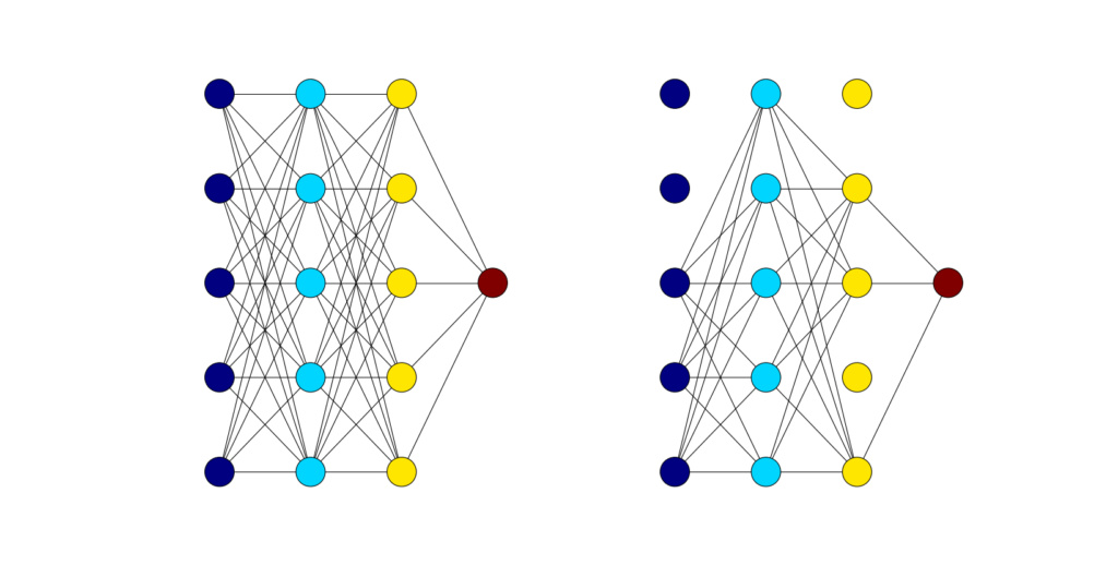
一个dropout 层有一个称为p的超参数,它仅仅是每个单元被保存在神经网络模型中进行迭代训练的概率。被保存的单位将其输出提供给下一层,而不被保存的单位则没有提供任何东西。下面是一个例子,展示了一个没有dropout的完全连接的神经网络和一个在迭代训练过程中dropout的完全连接的神经网络之间的区别:
dropout对LSTM层的内部的门来说并不是很好。某些关键记忆的丢失意味着一阶逻辑的复杂关系需要更多的时间与dropout,所以对于我们的LSTM层,我们将跳过内部的门的使用。这是Tensorflow的 DropoutWrapper对于循环层的默认实现。
第一步是标记化,用我们的GloVe字典把两个输入的句子变成一个向量序列。由于我们不能有效地使用在LSTM中传递的信息,所以我们将使用单词和最终输出的功能上的dropout,而不是在展开的LSTM神经网络部分的第一层和最后一层有效地使用dropout。
你可能注意到我们使用了一个双向RNN,它有两个不同的LSTM单元。这种形式的循环网络既向前又向后地运行输入数据,使得网络既能够独立又能相互之间对假设和证据进行审查。
LSTMs最终的输出将被传递到一套完整的连接层,然后,我们将得到一个实值的分数表明每种entailment的强度,结果。
为了测试精度并开始增加优化约束,我们需要展示TensorFlow如何计算准确预测标签的准确度或百分比。
我们还需要确定一个损失,以显示神经网络的运行状况。由于我们有分类分数和最优分数,所以这里的选择是使用来自TensorFlow的softmax损失的变化:tf.nn.softmax_cross_entropy_with_logits。我们增加了正则化的损失以帮助过度拟合,然后准备一个优化器来学习如何减少损失。
最后,训练神经网络。如果你安装了TQDM,可以使用它来跟踪神经网络训练的进度。
神经网络现在被训练。应该看到大约50 - 55%的准确性,可以通过仔细修改超参数和增加数据集的大小以包括整个训练集来改进。通常,这与训练时间的增加有关。
通过插入自己的句子,修改在notebook上代码:
最后,我们完成了模型的操作,结束会话以释放系统资源。
本文为编译作品,作者
https://www.oreilly.com/learning/textual-entailment-with-tensorflow
作为应用程序的一个组成部分,文本含义识别是有用的。例如,问答系统可以使用文本含义识别来验证存储信息的答案。其他自然语言处理系统(NLP)也发现类似的应用。
本文将引导你了解如何构建一个简单快捷的神经网络来执行使用TensorFlow.的文本含义识别。
在我们开始之前
除了安装 TensorFlow version 1.0之外,还要确保安装:
Jupyter
Numpy
Matplotlib
为了在神经网络训练中获得更多的进步,可以安装 TQDM,但这不是必需的。请访问GitHub上的这篇文章的代码和Jupyter笔记本(链接为https://github.com/Steven-Hewitt/Entailment-with-Tensorflow)。我们将使用斯坦福的SNLI数据集来进行我们的训练,使用Jupyter Notebook中的代码下载并提取我们需要的数据。如果这是你第一次使用TensorFlow,我建议你看看Aaron Schumacher的文章“Hello, Tensorflow”。
将从所有必要的输入开始,利用Jupyter Notebook显示图表和图像。
%matplotlib inline


import tensorflow as tf

import numpy as np

import matplotlib.pyplot as plt

import matplotlib.ticker as ticker

import urllib

import sys

import os

import zipfile
文本含义识别示例
在本节中,我们将通过一些文本含义识别的例子来说明positive, negative和 neutral entailment。首先,我们来看看positive entailment——例如,当你读到“Maurita and Jade both were at the scene of the car crash”时,你可以推断“Multiple people saw the accident”。在这个例句中,我们可以用第一个句子(也称为“文本”)证明第二句(也称为“假设”),这代表是positive entailment。鉴于莫丽塔和杰德都看到车祸,说明有多人看到。
让我们考虑另一个句子对。“在公园里和老人一起玩的两只狗”推导“那天公园里只有一只狗”。第一句话说有“两只狗”,那么就说明公园至少有两只狗,第二句话与这个观点相矛盾,所以是negative entailment。
最后,为了阐明neutral entailment,我们看“我和孩子们打棒球”和“孩子们爱吃冰淇淋”这两句话,打棒球和爱吃冰淇淋完全没有任何关系。我可以和冰淇淋爱好者打棒球,我也可以和不喜欢冰淇淋的人打棒球(两者都是可能的)。因此,第一句话没有说明第二句话的真实或虚假。
数字使用word vectorization来展示句子
对于神经网络来说,它们主要使用数字值工作。为了解决这个问题,我们需要用数字来表示我们的单词。这些数字意味着什么,例如,我们可以使用字母中的字符代码,但这并没有告诉我们任何关于它的含义(这意味着TensorFlow不得不做大量的工作来说明“dog”和“canine”是接近相同的概念)。将类似的意义转化为神经网络可以理解的过程,这个过程被称为word vectorization。
常用的创建word vectorization的方法是让每个单词表示一个非常高维空间中的一个点。具有相似含义的单词应该在这个空间中相对接近。这一点的演示在 word vectorization的TensorFlow教程中可以找到(链接地址是https://www.tensorflow.org/tutorials/word2vec)。
使用斯坦福的GloVe word vectorization+ SNLI数据集
我们不需要创建一个新的表达形式。如果通用数据不够用,可以用已经存在的一些很好的通用矢量表现形式和训练专业材料的方法。
我们将使用60亿的Wikipedia 2014 + Gigaword 5向量,因为它是最小并且最容易下载的。我们将以编程方式下载该文件,运行它可能需要一段时间(这是一个相当大的文件)。
与此同时,我们收集我们的textual entailment数据集:斯坦福大学SNLI数据集。
glove_zip_file = "glove.6B.zip"

glove_vectors_file = "glove.6B.50d.txt"


snli_zip_file = "snli_1.0.zip"

snli_dev_file = "snli_1.0_dev.txt"

snli_full_dataset_file = "snli_1.0_train.txt"
from six.moves.url.lib.request import urlretrieve


#large file - 862 MB

if (not os.path.isfile(glove_zip_file) and

    not os.path.isfile(glove_vectors_file)):

    urlretrieve ("http://nlp.stanford.edu/data/glove.6B.zip",

                 glove_zip_file)


#medium-sized file - 94.6 MB

if (not os.path.isfile(snli_zip_file) and

    not os.path.isfile(snli_dev_file)):

    urlretrieve ("https://nlp.stanford.edu/projects/snli/snli_1.0.zip",

                 snli_zip_file)
def unzip_single_file(zip_file_name, output_file_name):

    """

        If the outFile is already created, don't recreate

        If the outFile does not exist, create it from the zipFile

    """

    if not os.path.isfile(output_file_name):

        with open(output_file_name, 'wb') as out_file:

            with zipfile.ZipFile(zip_file_name) as zipped:

                for info in zipped.infolist():

                    if output_file_name in info.filename:

                        with zipped.open(info) as requested_file:

                            out_file.write(requested_file.read())

                            return


unzip_single_file(glove_zip_file, glove_vectors_file)

unzip_single_file(snli_zip_file, snli_dev_file)

# unzip_single_file(snli_zip_file, snli_full_dataset_file)
现在我们已经下载了GloVe向量,将它们加载到储存器中,将空间分隔的格式反序列化为Python字典:
glove_wordmap = {}

with open(glove_vectors_file, "r") as glove:

    for line in glove:

        name, vector = tuple(line.split(" ", 1))

        glove_wordmap[name] = np.fromstring(vector, sep=" ")
通过神经网络来处理句子。让我们从制作这个序列开始:
def sentence2sequence(sentence):

    """


    - Turns an input sentence into an (n,d) matrix,

        where n is the number of tokens in the sentence

        and d is the number of dimensions each word vector has.


      Tensorflow doesn't need to be used here, as simply

      turning the sentence into a sequence based off our

      mapping does not need the computational power that

      Tensorflow provides. Normal Python suffices for this task.

    """

    tokens = sentence.lower().split(" ")

    rows = []

    words = []

    #Greedy search for tokens

    for token in tokens:

        i = len(token)

        while len(token) > 0 and i > 0:

            word = token[:i]

            if word in glove_wordmap:

                rows.append(glove_wordmap[word])

                words.append(word)

                token = token[i:]

                i = len(token)

            else:

                i = i-1

    return rows, words
当计算机研究句子的时会看到什么
为了更好地理解word vectorization过程以及算机研究句子时所看到的东西,我们可以将这些向量表示为图像。使用notebook 将句子可视化。每一行表示一个词,而列表示word vectorization的个体维度。word vectorization是在根据单词与其他单词的关系进行训练的,实际上表示的含义是含糊不清的。但计算机能理解这种向量语言,这是最重要的部分。一般来说,在相同的位置上颜色相似的两个向量表示单词在意义上相似。
def visualize(sentence):

    rows, words = sentence2sequence(sentence)

    mat = np.vstack(rows)


    fig = plt.figure()

    ax = fig.add_subplot(111)

    shown = ax.matshow(mat, aspect="auto")

    ax.yaxis.set_major_locator(ticker.MultipleLocator(1))

    fig.colorbar(shown)


    ax.set_yticklabels([""]+words)

    plt.show()


visualize("The quick brown fox jumped over the lazy dog.")

visualize("The pretty flowers shone in the sunlight.")
与图像不同的是,句子有固有的顺序,且不受大小的约束,所以我们需要一种新的不完全连接前馈网络的神经网络类型,这是因为前馈网络占据一个输入值并且只需运行到产生一个输出,而我们需要循环。
Vanilla循环网络
Recurrent neural networks(RNNs)是神经网络的一种序列学习工具。这种类型的神经网络只有一层的隐藏输入,它被重复用于序列中的每个输入,以及传递给下一个输入计算的“memory”。
对序列中的每一个输入重复同样的计算,这意味着Recurrent neural networks的一个“层”可以被展开成许多层。这使得神经网络能够处理一个非常复杂的句子。TensorFlow有一个简单的RNN cell,BasicRNNCell的实现,它可以添加到你的TensorFlow中,如下图:
rnn_size = 64

rnn = tf.contrib.rnn.BasicRNNCell(rnn_size)
梯度消失问题
从理论上讲,神经网络将能够记住来自第一层的东西,甚至是一个早期句子的结尾。这种循环形式的主要问题是:在实践中,早期的数据被更新的并不重要的输入和信息完全淹没。Recurrent neural networks或者是带有标准隐藏单位的神经网络不能长时间维持信息。这个故障被称为梯度消失问题。
最简单的方法就是通过示例可视化。在最简单的情况下,输入和“memory”权重大致相同。数据的第一个输入将影响第一个输出的大约一半(另一半是启动“memory”),第二次输出的四分之一,然后是第三输出的八分之一,等等。
这意味着我们不能使用vanilla循环网络,如果我们想要对这两个句子进行追踪。解决方案是使用不同类型的循环网络层。也许最简单的就是长短期记忆层,也就是LSTM。
利用LSTM
在LSTM中,代替计算当前储存器时每次都使用相同方式的输入(xt),神经网络可以通过“输入门”(it)决定当前值对储存器的影响程度,并做出一个决定;通过被命名为“忘记门”(ft)的遗忘的存储器(ct)做出另外一个决定,根据储存器将哪些部分通过“输出门”(ot)发送到下一个时间步长(ht)做第三个决定。
这三个门的组合创造了一个选择:一个单一的LSTM节点,可以将信息保存在长期储存器中,也可以将信息保存在短期储存器中,但不能同时进行。短期记忆LSTMs训练的是相对开放的输入门,让大量的信息进来,也经常忘记很多;而长期记忆LSTMs有紧密的输入门,只允许非常小的,非常具体的信息进入。这种紧密性意味着它不会轻易失去它的信息,并且允许保存更长的时间。
总的来说,LSTMs是非常神秘的。不同LSTM节点在同一个神经网络可能会有彼此依赖但又截然不同的门。
为神经网络定义常量
我们不打算在我们的神经网络中使用 vanilla RNN层,所以我们会清除图表并添加一个LSTM层,默认情况下也包含TensorFlow。这将是我们神经网络的第一部分,定义神经网络的需要的所有常数:
#Constants setup

max_hypothesis_length, max_evidence_length = 30, 30

batch_size, vector_size, hidden_size = 128, 50, 64


lstm_size = hidden_size


weight_decay = 0.0001


learning_rate = 1


input_p, output_p = 0.5, 0.5


training_iterations_count = 100000


display_step = 10


def score_setup(row):

    convert_dict = {

      'entailment': 0,

      'neutral': 1,

      'contradiction': 2

    }

    score = np.zeros((3,))

    for x in range(1,6):

        tag = row["label"+str(x)]

        if tag in convert_dict: score[convert_dict[tag]] += 1

    return score / (1.0*np.sum(score))


def fit_to_size(matrix, shape):

    res = np.zeros(shape)

    slices = [slice(0,min(dim,shape[e])) for e, dim in enumerate(matrix.shape)]

    res[slices] = matrix[slices]

    return res
def split_data_into_scores():

    import csv

    with open("snli_1.0_dev.txt","r") as data:

        train = csv.DictReader(data, delimiter='\t')

        evi_sentences = []

        hyp_sentences = []

        labels = []

        scores = []

        for row in train:

            hyp_sentences.append(np.vstack(

                    sentence2sequence(row["sentence1"].lower())[0]))

            evi_sentences.append(np.vstack(

                    sentence2sequence(row["sentence2"].lower())[0]))

            labels.append(row["gold_label"])

            scores.append(score_setup(row))


        hyp_sentences = np.stack([fit_to_size(x, (max_hypothesis_length, vector_size))

                          for x in hyp_sentences])

        evi_sentences = np.stack([fit_to_size(x, (max_evidence_length, vector_size))

                          for x in evi_sentences])


        return (hyp_sentences, evi_sentences), labels, np.array(scores)


data_feature_list, correct_values, correct_scores = split_data_into_scores()


l_h, l_e = max_hypothesis_length, max_evidence_length

N, D, H = batch_size, vector_size, hidden_size

l_seq = l_h + l_e
我们还将重新设置图表,不包括我们之前添加的RNN单元。
tf.reset_default_graph()
使用TensorFlow定义我们的LSTM,它的使用方式如下:
lstm = tf.contrib.rnn.BasicLSTMCell(lstm_size)
实现dropout
如果我们只是简单地使用了LSTM层,而没有更多的东西,那么这个神经网络可能会读到很多普通的,无关紧要的词,比如“a”、“the”、和“and”。如果一个句子使用“an animal”这个短语,而另一个句子使用“the animal”,即使这些短语指的是同一个对象,神经网络也可能错误地认为它已经找到了negative entailment。
为了解决这个问题,我们需要调整一下,看看个别单词是否对整体有重要意义,我们通过一个叫“dropout”的过程来实现。dropout是神经网络设计中的一种正则化模式,它围绕着随机选择的隐藏和可见的单位。随着神经网络大小的增加,用来计算最终结果的参数个数也随着增加,如果一次训练全部,每个参数都会过度拟合。为了规范这一点,在训练中随机抽取神经网络中包含的部分,并在训练时临时调零,在实际使用过程中,它们的输出被适当地缩放。
“标准”(即完全连接)层上的dropout也是有用的,因为它有效地训练了多个较小的神经网络,然后在测试时间内组合它们。机器学习中的一个常数使自己比单个模型更好的方法就是组合多个模型,并且 dropout 用于将单个神经网络转换为共享一些节点的多个较小的神经网络。
一个dropout 层有一个称为p的超参数,它仅仅是每个单元被保存在神经网络模型中进行迭代训练的概率。被保存的单位将其输出提供给下一层,而不被保存的单位则没有提供任何东西。下面是一个例子,展示了一个没有dropout的完全连接的神经网络和一个在迭代训练过程中dropout的完全连接的神经网络之间的区别:
用于循环层的Tensorflow的DropoutWrapper
dropout对LSTM层的内部的门来说并不是很好。某些关键记忆的丢失意味着一阶逻辑的复杂关系需要更多的时间与dropout,所以对于我们的LSTM层,我们将跳过内部的门的使用。这是Tensorflow的 DropoutWrapper对于循环层的默认实现。
lstm_drop = tf.contrib.rnn.DropoutWrapper(lstm, input_p, output_p)
完成我们的模型
第一步是标记化,用我们的GloVe字典把两个输入的句子变成一个向量序列。由于我们不能有效地使用在LSTM中传递的信息,所以我们将使用单词和最终输出的功能上的dropout,而不是在展开的LSTM神经网络部分的第一层和最后一层有效地使用dropout。
你可能注意到我们使用了一个双向RNN,它有两个不同的LSTM单元。这种形式的循环网络既向前又向后地运行输入数据,使得网络既能够独立又能相互之间对假设和证据进行审查。
LSTMs最终的输出将被传递到一套完整的连接层,然后,我们将得到一个实值的分数表明每种entailment的强度,结果。
# N: The number of elements in each of our batches,

#   which we use to train subsets of data for efficiency's sake.

# l_h: The maximum length of a hypothesis, or the second sentence.  This is

#   used because training an RNN is extraordinarily difficult without

#   rolling it out to a fixed length.

# l_e: The maximum length of evidence, the first sentence.  This is used

#   because training an RNN is extraordinarily difficult without

#   rolling it out to a fixed length.

# D: The size of our used GloVe or other vectors.

hyp = tf.placeholder(tf.float32, [N, l_h, D], 'hypothesis')

evi = tf.placeholder(tf.float32, [N, l_e, D], 'evidence')

y = tf.placeholder(tf.float32, [N, 3], 'label')

# hyp: Where the hypotheses will be stored during training.

# evi: Where the evidences will be stored during training.

# y: Where correct scores will be stored during training.


# lstm_size: the size of the gates in the LSTM,

#    as in the first LSTM layer's initialization.

lstm_back = tf.contrib.rnn.BasicLSTMCell(lstm_size)

# lstm_back:  The LSTM used for looking backwards

#   through the sentences, similar to lstm.


# input_p: the probability that inputs to the LSTM will be retained at each

#   iteration of dropout.

# output_p: the probability that outputs from the LSTM will be retained at

#   each iteration of dropout.

lstm_drop_back = tf.contrib.rnn.DropoutWrapper(lstm_back, input_p, output_p)

# lstm_drop_back:  A dropout wrapper for lstm_back, like lstm_drop.


fc_initializer = tf.random_normal_initializer(stddev=0.1)

# fc_initializer: initial values for the fully connected layer's weights.

# hidden_size: the size of the outputs from each lstm layer.

#   Multiplied by 2 to account for the two LSTMs.

fc_weight = tf.get_variable('fc_weight', [2*hidden_size, 3],

                            initializer = fc_initializer)

# fc_weight: Storage for the fully connected layer's weights.

fc_bias = tf.get_variable('bias', [3])

# fc_bias: Storage for the fully connected layer's bias.


# tf.GraphKeys.REGULARIZATION_LOSSES:  A key to a collection in the graph

#   designated for losses due to regularization.

#   In this case, this portion of loss is regularization on the weights

#   for the fully connected layer.

tf.add_to_collection(tf.GraphKeys.REGULARIZATION_LOSSES,

                     tf.nn.l2_loss(fc_weight))


x = tf.concat([hyp, evi], 1) # N, (Lh+Le), d

# Permuting batch_size and n_steps

x = tf.transpose(x, [1, 0, 2]) # (Le+Lh), N, d

# Reshaping to (n_steps*batch_size, n_input)

x = tf.reshape(x, [-1, vector_size]) # (Le+Lh)*N, d

# Split to get a list of 'n_steps' tensors of shape (batch_size, n_input)

x = tf.split(x, l_seq,)


# x: the inputs to the bidirectional_rnn


# tf.contrib.rnn.static_bidirectional_rnn: Runs the input through

#   two recurrent networks, one that runs the inputs forward and one

#   that runs the inputs in reversed order, combining the outputs.

rnn_outputs, _, _ = tf.contrib.rnn.static_bidirectional_rnn(lstm, lstm_back,

                                                            x, dtype=tf.float32)

# rnn_outputs: the list of LSTM outputs, as a list.

#   What we want is the latest output, rnn_outputs[-1]


classification_scores = tf.matmul(rnn_outputs[-1], fc_weight) + fc_bias

# The scores are relative certainties for how likely the output matches

#   a certain entailment:

#     0: Positive entailment

#     1: Neutral entailment

#     2: Negative entailment
展示TensorFlow如何计算准确度
为了测试精度并开始增加优化约束,我们需要展示TensorFlow如何计算准确预测标签的准确度或百分比。
我们还需要确定一个损失,以显示神经网络的运行状况。由于我们有分类分数和最优分数,所以这里的选择是使用来自TensorFlow的softmax损失的变化:tf.nn.softmax_cross_entropy_with_logits。我们增加了正则化的损失以帮助过度拟合,然后准备一个优化器来学习如何减少损失。
with tf.variable_scope('Accuracy'):

    predicts = tf.cast(tf.argmax(classification_scores, 1), 'int32')

    y_label = tf.cast(tf.argmax(y, 1), 'int32')

    corrects = tf.equal(predicts, y_label)

    num_corrects = tf.reduce_sum(tf.cast(corrects, tf.float32))

    accuracy = tf.reduce_mean(tf.cast(corrects, tf.float32))


with tf.variable_scope("loss"):

    cross_entropy = tf.nn.softmax_cross_entropy_with_logits(

        logits = classification_scores, labels = y)

    loss = tf.reduce_mean(cross_entropy)

    total_loss = loss + weight_decay * tf.add_n(

        tf.get_collection(tf.GraphKeys.REGULARIZATION_LOSSES))


optimizer = tf.train.GradientDescentOptimizer(learning_rate)


opt_op = optimizer.minimize(total_loss)
训练神经网络
最后,训练神经网络。如果你安装了TQDM,可以使用它来跟踪神经网络训练的进度。
# Initialize variables

init = tf.global_variables_initializer()


# Use TQDM if installed

tqdm_installed = False

try:

    from tqdm import tqdm

    tqdm_installed = True

except:

    pass


# Launch the Tensorflow session

sess = tf.Session()

sess.run(init)


# training_iterations_count: The number of data pieces to train on in total

# batch_size: The number of data pieces per batch

training_iterations = range(0,training_iterations_count,batch_size)

if tqdm_installed:

    # Add a progress bar if TQDM is installed

    training_iterations = tqdm(training_iterations)


for i in training_iterations:


    # Select indices for a random data subset

    batch = np.random.randint(data_feature_list[0].shape[0], size=batch_size)


    # Use the selected subset indices to initialize the graph's

    #   placeholder values

    hyps, evis, ys = (data_feature_list[0][batch,:],

                      data_feature_list[1][batch,:],

                      correct_scores[batch])


    # Run the optimization with these initialized values

    sess.run([opt_op], feed_dict={hyp: hyps, evi: evis, y: ys})

    # display_step: how often the accuracy and loss should

    #   be tested and displayed.

    if (i/batch_size) % display_step == 0:

        # Calculate batch accuracy

        acc = sess.run(accuracy, feed_dict={hyp: hyps, evi: evis, y: ys})

        # Calculate batch loss

        tmp_loss = sess.run(loss, feed_dict={hyp: hyps, evi: evis, y: ys})

        # Display results

        print("Iter " + str(i/batch_size) + ", Minibatch Loss= " + \

              "{:.6f}".format(tmp_loss) + ", Training Accuracy= " + \

              "{:.5f}".format(acc))
神经网络现在被训练。应该看到大约50 - 55%的准确性,可以通过仔细修改超参数和增加数据集的大小以包括整个训练集来改进。通常,这与训练时间的增加有关。
通过插入自己的句子,修改在notebook上代码:
evidences = ["Maurita and Jade both were at the scene of the car crash."]


hypotheses = ["Multiple people saw the accident."]


sentence1 = [fit_to_size(np.vstack(sentence2sequence(evidence)[0]),

                         (30, 50)) for evidence in evidences]


sentence2 = [fit_to_size(np.vstack(sentence2sequence(hypothesis)[0]),

                         (30,50)) for hypothesis in hypotheses]


prediction = sess.run(classification_scores, feed_dict={hyp: (sentence1 * N),

                                                        evi: (sentence2 * N),

                                                        y: [[0,0,0]]*N})

print(["Positive", "Neutral", "Negative"][np.argmax(prediction[0])]+

      " entailment")
最后,我们完成了模型的操作,结束会话以释放系统资源。
sess.close()
本文为编译作品,作者
https://www.oreilly.com/learning/textual-entailment-with-tensorflow

欢迎关注ATYUN官方公众号
商务合作及内容投稿请联系邮箱:bd@atyun.com


广告


写评论取消
回复取消