


请先登录您的atyun账户,方可使用该功能

审核通过后即可使用此功能,请耐心等待~


Python机器学习的练习四:多元逻辑回归
2018年06月01日 由 xiaoshan.xiang 发表
791504
0
Python机器学习的练习系列共有八个部分:
Python机器学习的练习一:简单线性回归
Python机器学习的练习二:多元线性回归
Python机器学习的练习三:逻辑回归
Python机器学习的练习四:多元逻辑回归
Python机器学习的练习五:神经网络
Python机器学习的练习六:支持向量机
Python机器学习的练习七:K-Means聚类和主成分分析
Python机器学习的练习八:异常检测和推荐系统
在Python机器学习的练习第3部分中,我们实现了简单的和正则化的逻辑回归。但我们的解决方法有一个限制—它只适用于二进制分类。在本文中,我们将在之前的练习中扩展我们的解决方案,以处理多级分类问题。
在语法上快速标注,为了显示语句的输出,我在代码块中附加了一个“>”,以表明它是运行先前语句的结果。如果结果很长(超过1-2行),那么我就把它粘贴在代码块的另一个单独的块中。希望可以清楚的说明哪些语句是输入,哪些是输出。
此练习中的任务是使用逻辑回归来识别手写数字(0-9)。首先加载数据集。与前面的示例不同,我们的数据文件是MATLAB的本体格式,不能被pandas自动识别,所以把它加载在Python中需要使用SciPy utility。
快速检查加载到储存器中的矩阵的形状
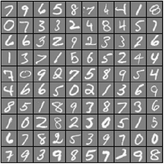
我们已经加载了我们的数据。图像在martix X 被表现为400维的向量。这400个“特征”是原始20x20图像中每个像素的灰度强度。类标签在向量y中表示图像中数字的数字类。下面的图片给出了一些数字的例子。每个带有白色手写数字的灰色框代表我们数据集中400维的行。
我们的第一个任务是修改逻辑回归的实现以完全向量化(即没有“for”循环),这是因为矢量化代码除了简洁扼要,还能够利用线性代数优化,并且比迭代代码快得多。我们在练习二中的成本函数实现已经向量化。所以我们在这里重复使用相同的实现。请注意,我们正在跳到最终的正则化版本。
这个成本函数与我们在先前练习中创建的函数是相同的,如果你不确定我们如何做到这一点,在运行之前查看以前的文章。
接下来,我们需要计算梯度的函数。我们已经在前面的练习中定义了它,我们在更新步骤中需要去掉“for”循环。这是可供参考的原始代码:
梯度函数详细的阐述了如何改变一个参数,以获得一个比之前好的答案。如果你不熟悉线性代数,这一系列运作背后的数学是很难理解的。
现在我们需要创建一个不使用任何循环的梯度函数的版本。在我们的新版本中,我们将去掉“for”循环,并使用线性代数(除了截距参数,它需要单独计算)计算每个参数的梯度。
还要注意,我们将数据结构转换为NumPy矩阵。这样做是为了使代码看起来更像Octave,而不是数组,这是因为矩阵自动遵循矩阵运算规则与element-wise运算。我们在下面的例子中使用矩阵。
现在我们已经定义了成本和梯度函数,接下来创建一个分类器。对于本章练习的任务,我们有10个可能的分类,由于逻辑回归一次只能区分两个类别,我们需要一个方法去处理多类别场景。在这个练习中我们的任务是实现一对多的分类,其中k个不同类的标签导致了k个分类器,每个分类器在“class i”和“not class i”之间做决定。我们将在一个函数中完成分类器的训练,计算10个分类器的最终权重,并将权重返回作为k X(n + 1)数组,其中n是参数数。
这里需要注意的几点:首先,我们为theta添加了一个额外的参数(带有一列训练数据)以计算截距项。其次,我们将y从类标签转换为每个分类器的二进制值(要么是I类,要么不是I类)。最后,我们使用SciPy的较新优化API来最小化每个分类器的成本函数。API利用目标函数、初始参数集、优化方法和jacobian(梯度)函数,将优化程序找到的参数分配给参数数组。
实现向量化代码的一个更具挑战性的部分是正确地写入所有的矩阵交互,所以通过查看正在使用的数组/矩阵的形状来做一些健全性检查是有用的,我们来看看上面的函数中使用的一些数据结构。
注意,theta是一维数组,所以当它被转换为计算梯度的代码中的矩阵时,它变成一个(1×401)矩阵。 我们还要检查y中的类标签,以确保它们看起来像我们期望的。
确保函数正常运行,并获得一些合理的输出。
最后一步是使用训练过的分类器预测每个图像的标签。对于这一步骤,对于每个训练实例(使用矢量化代码),我们将计算每个类的类概率,并将输出类标签分配给具有最高概率的类。
现在我们可以使用predict_all函数为每个实例生成类预测,并了解分类器的工作情况。
接近98%,相当不错,逻辑回归是一个相对简单的方法。
Python机器学习的练习一:简单线性回归
Python机器学习的练习二:多元线性回归
Python机器学习的练习三:逻辑回归
Python机器学习的练习四:多元逻辑回归
Python机器学习的练习五:神经网络
Python机器学习的练习六:支持向量机
Python机器学习的练习七:K-Means聚类和主成分分析
Python机器学习的练习八:异常检测和推荐系统
在Python机器学习的练习第3部分中,我们实现了简单的和正则化的逻辑回归。但我们的解决方法有一个限制—它只适用于二进制分类。在本文中,我们将在之前的练习中扩展我们的解决方案,以处理多级分类问题。
在语法上快速标注,为了显示语句的输出,我在代码块中附加了一个“>”,以表明它是运行先前语句的结果。如果结果很长(超过1-2行),那么我就把它粘贴在代码块的另一个单独的块中。希望可以清楚的说明哪些语句是输入,哪些是输出。
此练习中的任务是使用逻辑回归来识别手写数字(0-9)。首先加载数据集。与前面的示例不同,我们的数据文件是MATLAB的本体格式,不能被pandas自动识别,所以把它加载在Python中需要使用SciPy utility。
import numpy as np

import pandas as pd

import matplotlib.pyplot as plt

from scipy.io import loadmat

%matplotlib inline


data = loadmat('data/ex3data1.mat')

data

{'X': array([[ 0.,  0.,  0., ...,  0.,  0.,  0.],

        [ 0.,  0.,  0., ...,  0.,  0.,  0.],

        [ 0.,  0.,  0., ...,  0.,  0.,  0.],

        ...,

        [ 0.,  0.,  0., ...,  0.,  0.,  0.],

        [ 0.,  0.,  0., ...,  0.,  0.,  0.],

        [ 0.,  0.,  0., ...,  0.,  0.,  0.]]),

 '__globals__': [],

 '__header__': 'MATLAB 5.0 MAT-file, Platform: GLNXA64, Created on: Sun Oct 16 13:09:09 2011',

 '__version__': '1.0',

 'y': array([[10],

        [10],

        [10],

        ...,

        [ 9],

        [ 9],

        [ 9]], dtype=uint8)}
快速检查加载到储存器中的矩阵的形状
data['X'].shape, data['y'].shape


> ((5000L, 400L), (5000L, 1L))
我们已经加载了我们的数据。图像在martix X 被表现为400维的向量。这400个“特征”是原始20x20图像中每个像素的灰度强度。类标签在向量y中表示图像中数字的数字类。下面的图片给出了一些数字的例子。每个带有白色手写数字的灰色框代表我们数据集中400维的行。
我们的第一个任务是修改逻辑回归的实现以完全向量化(即没有“for”循环),这是因为矢量化代码除了简洁扼要,还能够利用线性代数优化,并且比迭代代码快得多。我们在练习二中的成本函数实现已经向量化。所以我们在这里重复使用相同的实现。请注意,我们正在跳到最终的正则化版本。
def sigmoid(z):

    return 1 / (1 + np.exp(-z))


def cost(theta, X, y, learningRate):

    theta = np.matrix(theta)

    X = np.matrix(X)

    y = np.matrix(y)

    first = np.multiply(-y, np.log(sigmoid(X * theta.T)))

    second = np.multiply((1 - y), np.log(1 - sigmoid(X * theta.T)))

    reg = (learningRate / 2 * len(X)) * np.sum(np.power(theta[:,1:theta.shape[1]], 2))

    return np.sum(first - second) / (len(X)) + reg
这个成本函数与我们在先前练习中创建的函数是相同的,如果你不确定我们如何做到这一点,在运行之前查看以前的文章。
接下来,我们需要计算梯度的函数。我们已经在前面的练习中定义了它,我们在更新步骤中需要去掉“for”循环。这是可供参考的原始代码:
def gradient_with_loop(theta, X, y, learningRate):

    theta = np.matrix(theta)

    X = np.matrix(X)

    y = np.matrix(y)


    parameters = int(theta.ravel().shape[1])

    grad = np.zeros(parameters)


    error = sigmoid(X * theta.T) - y


    for i in range(parameters):

        term = np.multiply(error, X[:,i])


        if (i == 0):

            grad[i] = np.sum(term) / len(X)

        else:

            grad[i] = (np.sum(term) / len(X)) + ((learningRate / len(X)) * theta[:,i])


    return grad
梯度函数详细的阐述了如何改变一个参数,以获得一个比之前好的答案。如果你不熟悉线性代数,这一系列运作背后的数学是很难理解的。
现在我们需要创建一个不使用任何循环的梯度函数的版本。在我们的新版本中,我们将去掉“for”循环,并使用线性代数(除了截距参数,它需要单独计算)计算每个参数的梯度。
还要注意,我们将数据结构转换为NumPy矩阵。这样做是为了使代码看起来更像Octave,而不是数组,这是因为矩阵自动遵循矩阵运算规则与element-wise运算。我们在下面的例子中使用矩阵。
def gradient(theta, X, y, learningRate):

    theta = np.matrix(theta)

    X = np.matrix(X)

    y = np.matrix(y)


    parameters = int(theta.ravel().shape[1])

    error = sigmoid(X * theta.T) - y


    grad = ((X.T * error) / len(X)).T + ((learningRate / len(X)) * theta)


    # intercept gradient is not regularized

    grad[0, 0] = np.sum(np.multiply(error, X[:,0])) / len(X)


    return np.array(grad).ravel()
现在我们已经定义了成本和梯度函数,接下来创建一个分类器。对于本章练习的任务,我们有10个可能的分类,由于逻辑回归一次只能区分两个类别,我们需要一个方法去处理多类别场景。在这个练习中我们的任务是实现一对多的分类,其中k个不同类的标签导致了k个分类器,每个分类器在“class i”和“not class i”之间做决定。我们将在一个函数中完成分类器的训练,计算10个分类器的最终权重,并将权重返回作为k X(n + 1)数组,其中n是参数数。
from scipy.optimize import minimize


def one_vs_all(X, y, num_labels, learning_rate):

    rows = X.shape[0]

    params = X.shape[1]


    # k X (n + 1) array for the parameters of each of the k classifiers

    all_theta = np.zeros((num_labels, params + 1))


    # insert a column of ones at the beginning for the intercept term

    X = np.insert(X, 0, values=np.ones(rows), axis=1)


    # labels are 1-indexed instead of 0-indexed

    for i in range(1, num_labels + 1):

        theta = np.zeros(params + 1)

        y_i = np.array([1 if label == i else 0 for label in y])

        y_i = np.reshape(y_i, (rows, 1))


        # minimize the objective function

        fmin = minimize(fun=cost, x0=theta, args=(X, y_i, learning_rate), method='TNC', jac=gradient)

        all_theta[i-1,:] = fmin.x


    return all_theta
这里需要注意的几点:首先,我们为theta添加了一个额外的参数(带有一列训练数据)以计算截距项。其次,我们将y从类标签转换为每个分类器的二进制值(要么是I类,要么不是I类)。最后,我们使用SciPy的较新优化API来最小化每个分类器的成本函数。API利用目标函数、初始参数集、优化方法和jacobian(梯度)函数,将优化程序找到的参数分配给参数数组。
实现向量化代码的一个更具挑战性的部分是正确地写入所有的矩阵交互,所以通过查看正在使用的数组/矩阵的形状来做一些健全性检查是有用的,我们来看看上面的函数中使用的一些数据结构。
rows = data['X'].shape[0]

params = data['X'].shape[1]


all_theta = np.zeros((10, params + 1))


X = np.insert(data['X'], 0, values=np.ones(rows), axis=1)


theta = np.zeros(params + 1)


y_0 = np.array([1 if label == 0 else 0 for label in data['y']])

y_0 = np.reshape(y_0, (rows, 1))


X.shape, y_0.shape, theta.shape, all_theta.shape


> ((5000L, 401L), (5000L, 1L), (401L,), (10L, 401L))
注意,theta是一维数组,所以当它被转换为计算梯度的代码中的矩阵时,它变成一个(1×401)矩阵。 我们还要检查y中的类标签,以确保它们看起来像我们期望的。
np.unique(data['y'])


> array([ 1,  2,  3,  4,  5,  6,  7,  8,  9, 10], dtype=uint8)
确保函数正常运行,并获得一些合理的输出。
all_theta = one_vs_all(data['X'], data['y'], 10, 1)

all_theta
array([[ -5.79312170e+00,   0.00000000e+00,   0.00000000e+00, ...,

          1.22140973e-02,   2.88611969e-07,   0.00000000e+00],

       [ -4.91685285e+00,   0.00000000e+00,   0.00000000e+00, ...,

          2.40449128e-01,  -1.08488270e-02,   0.00000000e+00],

       [ -8.56840371e+00,   0.00000000e+00,   0.00000000e+00, ...,

         -2.59241796e-04,  -1.12756844e-06,   0.00000000e+00],

       ...,

       [ -1.32641613e+01,   0.00000000e+00,   0.00000000e+00, ...,

         -5.63659404e+00,   6.50939114e-01,   0.00000000e+00],

       [ -8.55392716e+00,   0.00000000e+00,   0.00000000e+00, ...,

         -2.01206880e-01,   9.61930149e-03,   0.00000000e+00],

       [ -1.29807876e+01,   0.00000000e+00,   0.00000000e+00, ...,

          2.60651472e-04,   4.22693052e-05,   0.00000000e+00]])
最后一步是使用训练过的分类器预测每个图像的标签。对于这一步骤,对于每个训练实例(使用矢量化代码),我们将计算每个类的类概率,并将输出类标签分配给具有最高概率的类。
def predict_all(X, all_theta):

    rows = X.shape[0]

    params = X.shape[1]

    num_labels = all_theta.shape[0]


    # same as before, insert ones to match the shape

    X = np.insert(X, 0, values=np.ones(rows), axis=1)


    # convert to matrices

    X = np.matrix(X)

    all_theta = np.matrix(all_theta)


    # compute the class probability for each class on each training instance

    h = sigmoid(X * all_theta.T)


    # create array of the index with the maximum probability

    h_argmax = np.argmax(h, axis=1)


    # because our array was zero-indexed we need to add one for the true label prediction

    h_argmax = h_argmax + 1


    return h_argmax
现在我们可以使用predict_all函数为每个实例生成类预测,并了解分类器的工作情况。
y_pred = predict_all(data['X'], all_theta)

correct = [1 if a == b else 0 for (a, b) in zip(y_pred, data['y'])]

accuracy = (sum(map(int, correct)) / float(len(correct)))

print 'accuracy = {0}%'.format(accuracy * 100)


> accuracy = 97.58%
接近98%,相当不错,逻辑回归是一个相对简单的方法。

欢迎关注ATYUN官方公众号
商务合作及内容投稿请联系邮箱:bd@atyun.com


广告


广告

写评论取消
回复取消