


请先登录您的atyun账户,方可使用该功能

审核通过后即可使用此功能,请耐心等待~


神经网络学习指南: 生成对抗样本
2018年06月01日 由 yining 发表
549736
0
为神经网络生成对抗样本是非常容易的,但是你需要格外小心那些小的,精心设计过的对输入的干扰,因为它们会导致神经网络错误地分类输入(input)。
在这篇文章中,我们将简单介绍生成对抗样本的算法,并将在TensorFlow中实现攻击的过程,以生产一个鲁棒性对抗样本。生成对抗样本的论文地址:https://arxiv.org/pdf/1707.07397.pdf
这篇文章会应用到开源Web应用程序Jupyter notebook。下载地址:http://www.anishathalye.com/media/2017/07/25/adversarial.ipynb

我们选择攻击一个在ImageNet上受过训练的Inception v3网络。在本节中,我们将从TF-slim图像分类库加载一个预先训练的网络。
首先,我们设置了输入图像。我们使用一个tf.Variable而不是tf.placeholder,因为我们需要将它变成可训练的。
接下来,我们加载 Inception v3 模型。
接下来,我们会加载预先训练过的权值。Inception v3的精度度将达到93.9%。
然后,我们编写一些代码来显示图像,对其进行分类,并显示分类结果。
给定一个图像x,我们的神经网络输出一个概率,分布在标签P(y∣x)上。当我们设计一个对抗输入时,我们想要找到一个x^,其中logP(y^∣x^)是目标labely ^ ℓ ∞
在这个框架中,一个对抗样本是约束优化问题的解决方案,我们可以使用反向传播算法和投影梯度下降法来解决这个问题。算法很简单:从初始化开始我们的对抗样本为x ^ ← x
1.x^←x^+α⋅∇logP(y^∣x^)
2.x^←clip(x^,x−ϵ,x+ϵ)
我们从最简单的部分开始:编写一个用于初始化的TensorFlow op。
接下来,我们编写梯度下降步骤,以最大化目标类的log概率(或等价地,将交叉熵(cross entropy)最小化)。
然后,我们编写预测步骤,以使我们的对抗样本与原始图像保持接近。此外,我们截取[0,1]以保持其有效的图像。
最后,我们准备生成一个对抗样本。我们任意选择“guacamole”(imagenet class 924)作为我们的目标类。
这种对抗图像与原始的图像没有视觉上的区别,然而,它却以一个非常高的概率被归类为 “guacamole”!
现在,让我们来看看一个更高级的样本。我们采取的方法是生成鲁棒性对抗样本来发现花猫图像的一个单一的干扰,这个干扰在一些选择的变换的分布中同时也是具有对抗性的。我们可以选择任何可微变换的分布;在这篇文章中,我们将生成一个单一的鲁棒性对抗输入,可以通过θ∈[−π/4,π/4]进行旋转。
在我们进行下一步之前,检查一下我们之前的样本是否在我们旋转它的时候仍然是具有对抗性的,例如把一个角度设定为θ=π/8。
看起来我们最初的对抗样本并不是旋转不变的!那么,我们如何让一个对抗样本对一个转换的分布产生鲁棒性呢?
首先,给定一些转换T的分布,我们可以使E t ∼ T log P ( y ^ ∣ t ( x ^ ) )
比起手动执行梯度采样,可以用一个小技巧来让TensorFlow为我们采样:我们可以对基于采样的梯度下降模型进行建模,而不是从分布中随机抽取样本,然后在分类之前转换它们的输入。
我们可以重新使用assign_op和project_step,尽管我们必须为这个新目标编写一个新的optim_step。
最后,我们准备运行PGD来生成我们的对抗输入。与前面的例子一样,我们再次选择“guacamole”作为我们的目标类。
这个对抗图像被高度自信地归类为“guacamole”,即使它被旋转了!
研究一下我们在整个角度范围内生成的鲁棒对抗样本的旋转不变性,让P(y^∣x^)除以θ∈[−π/4,π/4]。
我们可以看到,这是非常有效果的!
此文为编译作品,原网站:http://www.anishathalye.com/2017/07/25/synthesizing-adversarial-examples/#adversarial-examples
在这篇文章中,我们将简单介绍生成对抗样本的算法,并将在TensorFlow中实现攻击的过程,以生产一个鲁棒性对抗样本。生成对抗样本的论文地址:https://arxiv.org/pdf/1707.07397.pdf
这篇文章会应用到开源Web应用程序Jupyter notebook。下载地址:http://www.anishathalye.com/media/2017/07/25/adversarial.ipynb
设置
我们选择攻击一个在ImageNet上受过训练的Inception v3网络。在本节中,我们将从TF-slim图像分类库加载一个预先训练的网络。
import tensorflow as tf

import tensorflow.contrib.slim as slim

import tensorflow.contrib.slim.nets as nets
tf.logging.set_verbosity(tf.logging.ERROR)

sess = tf.InteractiveSession()
首先,我们设置了输入图像。我们使用一个tf.Variable而不是tf.placeholder,因为我们需要将它变成可训练的。
image = tf.Variable(tf.zeros((299, 299, 3)))
接下来,我们加载 Inception v3 模型。
def inception(image, reuse):


preprocessed = tf.multiply(tf.subtract(tf.expand_dims(image, 0), 0.5), 2.0)


arg_scope = nets.inception.inception_v3_arg_scope(weight_decay=0.0)


with slim.arg_scope(arg_scope):


logits, _ = nets.inception.inception_v3(


preprocessed, 1001, is_training=False, reuse=reuse)


logits = logits[:,1:] # ignore background class


probs = tf.nn.softmax(logits) # probabilities


return logits, probs


logits, probs = inception(image, reuse=False)
接下来,我们会加载预先训练过的权值。Inception v3的精度度将达到93.9%。
import tempfile

from urllib.request import urlretrieve

import tarfile

import os
data_dir = tempfile.mkdtemp()

inception_tarball, _ = urlretrieve(

    'http://download.tensorflow.org/models/inception_v3_2016_08_28.tar.gz')

tarfile.open(inception_tarball, 'r:gz').extractall(data_dir)
restore_vars = [

    var for var in tf.global_variables()

    if var.name.startswith('InceptionV3/')

]

saver = tf.train.Saver(restore_vars)

saver.restore(sess, os.path.join(data_dir, 'inception_v3.ckpt'))
然后,我们编写一些代码来显示图像,对其进行分类,并显示分类结果。
import json

import matplotlib.pyplot as plt
imagenet_json, _ = urlretrieve(

    'http://www.anishathalye.com/media/2017/07/25/imagenet.json')

with open(imagenet_json) as f:

    imagenet_labels = json.load(f)
def classify(img, correct_class=None, target_class=None):

    fig, (ax1, ax2) = plt.subplots(1, 2, figsize=(10, 8))

    fig.sca(ax1)

    p = sess.run(probs, feed_dict={image: img})[0]

    ax1.imshow(img)

    fig.sca(ax1)


    topk = list(p.argsort()[-10:][::-1])

    topprobs = p[topk]

    barlist = ax2.bar(range(10), topprobs)

    if target_class in topk:

        barlist[topk.index(target_class)].set_color('r')

    if correct_class in topk:

        barlist[topk.index(correct_class)].set_color('g')

    plt.sca(ax2)

    plt.ylim([0, 1.1])

    plt.xticks(range(10),

               [imagenet_labels[i][:15] for i in topk],

               rotation='vertical')

    fig.subplots_adjust(bottom=0.2)

    plt.show()
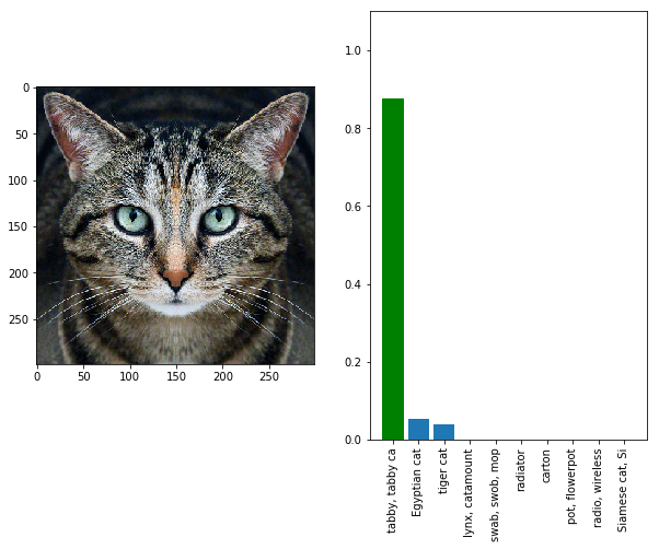
样本图像
加载样本图像并确保它被正确的分类。
import PIL

import numpy as np
img_path, _ = urlretrieve('http://www.anishathalye.com/media/2017/07/25/cat.jpg')

img_class = 281

img = PIL.Image.open(img_path)

big_dim = max(img.width, img.height)

wide = img.width > img.height

new_w = 299 if not wide else int(img.width * 299 / img.height)

new_h = 299 if wide else int(img.height * 299 / img.width)

img = img.resize((new_w, new_h)).crop((0, 0, 299, 299))

img = (np.asarray(img) / 255.0).astype(np.float32)
classify(img, correct_class=img_class)
对抗样本
给定一个图像x,我们的神经网络输出一个概率,分布在标签P(y∣x)上。当我们设计一个对抗输入时,我们想要找到一个x^,其中logP(y^∣x^)是目标label
在这个框架中,一个对抗样本是约束优化问题的解决方案,我们可以使用反向传播算法和投影梯度下降法来解决这个问题。算法很简单:从初始化开始我们的对抗样本为
1.x^←x^+α⋅∇logP(y^∣x^)
2.x^←clip(x^,x−ϵ,x+ϵ)
初始化
我们从最简单的部分开始:编写一个用于初始化的TensorFlow op。
x = tf.placeholder(tf.float32, (299, 299, 3))


x_hat = image # our trainable adversarial input

assign_op = tf.assign(x_hat, x)
梯度下降法步骤
接下来,我们编写梯度下降步骤,以最大化目标类的log概率(或等价地,将交叉熵(cross entropy)最小化)。
learning_rate = tf.placeholder(tf.float32, ())

y_hat = tf.placeholder(tf.int32, ())


labels = tf.one_hot(y_hat, 1000)

loss = tf.nn.softmax_cross_entropy_with_logits(logits=logits, labels=[labels])

optim_step = tf.train.GradientDescentOptimizer(

    learning_rate).minimize(loss, var_list=[x_hat])
预测步骤
然后,我们编写预测步骤,以使我们的对抗样本与原始图像保持接近。此外,我们截取[0,1]以保持其有效的图像。
epsilon = tf.placeholder(tf.float32, ())


below = x - epsilon

above = x + epsilon

projected = tf.clip_by_value(tf.clip_by_value(x_hat, below, above), 0, 1)

with tf.control_dependencies([projected]):

    project_step = tf.assign(x_hat, projected)
执行
最后,我们准备生成一个对抗样本。我们任意选择“guacamole”(imagenet class 924)作为我们的目标类。
demo_epsilon = 2.0/255.0 # a really small perturbation

demo_lr = 1e-1

demo_steps = 100

demo_target = 924 # "guacamole"


# initialization step

sess.run(assign_op, feed_dict={x: img})


# projected gradient descent

for i in range(demo_steps):

    # gradient descent step

    _, loss_value = sess.run(

        [optim_step, loss],

        feed_dict={learning_rate: demo_lr, y_hat: demo_target})

    # project step

    sess.run(project_step, feed_dict={x: img, epsilon: demo_epsilon})

    if (i+1) % 10 == 0:

        print('step %d, loss=%g' % (i+1, loss_value))


adv = x_hat.eval() # retrieve the adversarial example

step 10, loss=4.18923

step 20, loss=0.580237

step 30, loss=0.0322334

step 40, loss=0.0209522

step 50, loss=0.0159688

step 60, loss=0.0134457

step 70, loss=0.0117799

step 80, loss=0.0105757

step 90, loss=0.00962179

step 100, loss=0.00886694
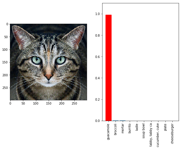
这种对抗图像与原始的图像没有视觉上的区别,然而,它却以一个非常高的概率被归类为 “guacamole”!
classify(adv, correct_class=img_class, target_class=demo_target)
鲁棒性对抗样本
现在,让我们来看看一个更高级的样本。我们采取的方法是生成鲁棒性对抗样本来发现花猫图像的一个单一的干扰,这个干扰在一些选择的变换的分布中同时也是具有对抗性的。我们可以选择任何可微变换的分布;在这篇文章中,我们将生成一个单一的鲁棒性对抗输入,可以通过θ∈[−π/4,π/4]进行旋转。
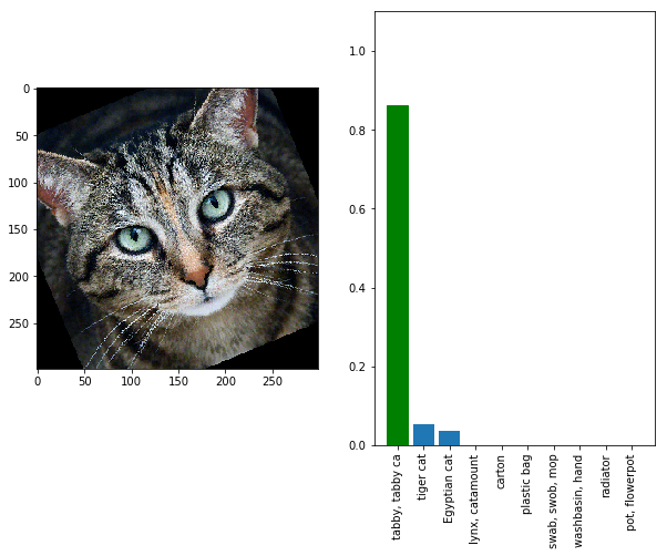
在我们进行下一步之前,检查一下我们之前的样本是否在我们旋转它的时候仍然是具有对抗性的,例如把一个角度设定为θ=π/8。
ex_angle = np.pi/8


angle = tf.placeholder(tf.float32, ())

rotated_image = tf.contrib.image.rotate(image, angle)

rotated_example = rotated_image.eval(feed_dict={image: adv, angle: ex_angle})

classify(rotated_example, correct_class=img_class, target_class=demo_target)
看起来我们最初的对抗样本并不是旋转不变的!那么,我们如何让一个对抗样本对一个转换的分布产生鲁棒性呢?
首先,给定一些转换T的分布,我们可以使
比起手动执行梯度采样,可以用一个小技巧来让TensorFlow为我们采样:我们可以对基于采样的梯度下降模型进行建模,而不是从分布中随机抽取样本,然后在分类之前转换它们的输入。
num_samples = 10

average_loss = 0

for i in range(num_samples):

    rotated = tf.contrib.image.rotate(

        image, tf.random_uniform((), minval=-np.pi/4, maxval=np.pi/4))

    rotated_logits, _ = inception(rotated, reuse=True)

    average_loss += tf.nn.softmax_cross_entropy_with_logits(

        logits=rotated_logits, labels=labels) / num_samples
我们可以重新使用assign_op和project_step,尽管我们必须为这个新目标编写一个新的optim_step。
optim_step = tf.train.GradientDescentOptimizer(

    learning_rate).minimize(average_loss, var_list=[x_hat])
最后,我们准备运行PGD来生成我们的对抗输入。与前面的例子一样,我们再次选择“guacamole”作为我们的目标类。
demo_epsilon = 8.0/255.0 # still a pretty small perturbation

demo_lr = 2e-1

demo_steps = 300

demo_target = 924 # "guacamole"


# initialization step

sess.run(assign_op, feed_dict={x: img})


# projected gradient descent

for i in range(demo_steps):

    # gradient descent step

    _, loss_value = sess.run(

        [optim_step, average_loss],

        feed_dict={learning_rate: demo_lr, y_hat: demo_target})

    # project step

    sess.run(project_step, feed_dict={x: img, epsilon: demo_epsilon})

    if (i+1) % 50 == 0:

        print('step %d, loss=%g' % (i+1, loss_value))


adv_robust = x_hat.eval() # retrieve the adversarial example
step 50, loss=0.0804289

step 100, loss=0.0270499

step 150, loss=0.00771527

step 200, loss=0.00350717

step 250, loss=0.00656128

step 300, loss=0.00226182
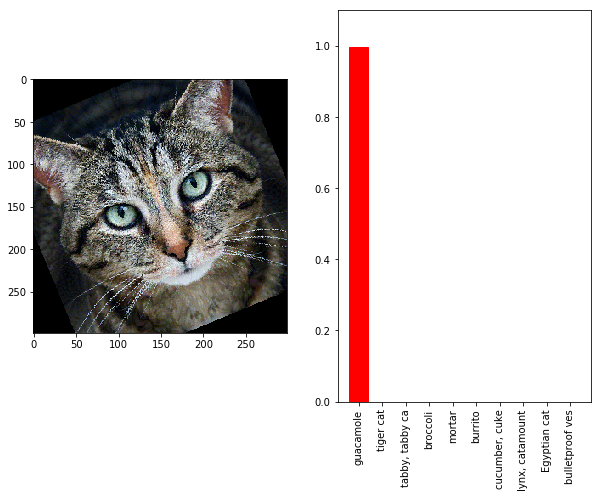
这个对抗图像被高度自信地归类为“guacamole”,即使它被旋转了!
rotated_example = rotated_image.eval(feed_dict={image: adv_robust, angle: ex_angle})

classify(rotated_example, correct_class=img_class, target_class=demo_target)
评估
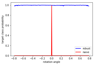
研究一下我们在整个角度范围内生成的鲁棒对抗样本的旋转不变性,让P(y^∣x^)除以θ∈[−π/4,π/4]。
thetas = np.linspace(-np.pi/4, np.pi/4, 301)


p_naive = []

p_robust = []

for theta in thetas:

    rotated = rotated_image.eval(feed_dict={image: adv_robust, angle: theta})

    p_robust.append(probs.eval(feed_dict={image: rotated})[0][demo_target])


    rotated = rotated_image.eval(feed_dict={image: adv, angle: theta})

    p_naive.append(probs.eval(feed_dict={image: rotated})[0][demo_target])


robust_line, = plt.plot(thetas, p_robust, color='b', linewidth=2, label='robust')

naive_line, = plt.plot(thetas, p_naive, color='r', linewidth=2, label='naive')

plt.ylim([0, 1.05])

plt.xlabel('rotation angle')

plt.ylabel('target class probability')

plt.legend(handles=[robust_line, naive_line], loc='lower right')

plt.show()
我们可以看到,这是非常有效果的!
此文为编译作品,原网站:http://www.anishathalye.com/2017/07/25/synthesizing-adversarial-examples/#adversarial-examples

欢迎关注ATYUN官方公众号
商务合作及内容投稿请联系邮箱:bd@atyun.com


广告


写评论取消
回复取消