


使用Keras集成卷积神经网络的入门级教程
介绍
在统计学和机器学习中,组合使用多种学习算法往往比单独的任何的学习算法更能获得好的预测性能。与统计力学中的统计集成不同(通常是无穷大),机器学习的集成由具体的有限的替代模型集合构成,但通常在这些备选方案中存在更灵活的结构。
使用集成主要是为了找到一个不一定包含在它所建立的模型的假设空间内的假设。从经验来看,当模型之间存在差异显著时,集成通常会产生更好的结果。
动机
如果你看过一些大型机器学习竞赛的结果,你很可能会发现,最好的结果是往往是由集成模型取得而不是由单一模型来实现。例如,ILSVRC2015(2015年大规模视觉识别挑战赛)得分最高的单一模型架构排在第13。前12名被各种各样的集成模型占据。
因为我暂时还没有看到关于这方面的教程,所以我决定自己制作关于这个主题的指南。
我将使用Keras的Functional API,创建三个小型CNN(与ResNet50,Inception等相比)。我分别在CIFAR-10训练数据集上训练每个模型。然后使用测试集分别评估。之后,我会把这三个模型集成在一起,并对其进行评估。我预计这个集成模型在测试集上的表现会比集成中任何一个单独的模型好。
集成有很多不同类型,堆叠(stacking)就是其中之一。它是比较常见的类型之一,理论上可以代表任何其他的集成技术。堆叠涉及训练一个学习算法以结合其他几种学习算法的预测。在这里,我将使用最简单的堆叠形式之一,它涉及到在集成中平均输出模型的输出。由于平均不需要任何参数,所以不需要训练这个集成(只有它的模型需要训练)。
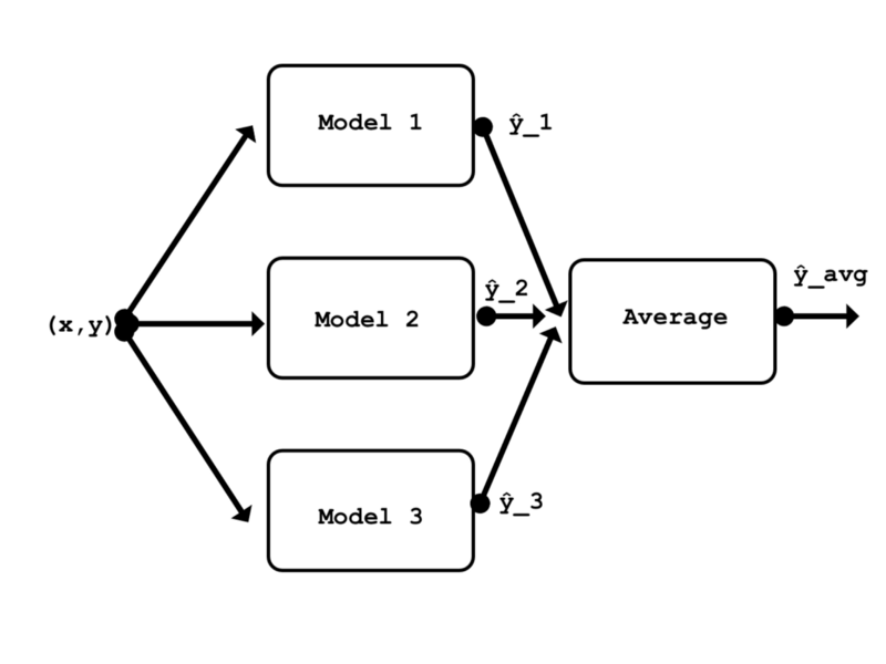
本文的集成概括图
准备数据
首先,导入依赖关系。
from keras.models import Model, Input

from keras.layers import Conv2D, MaxPooling2D, GlobalAveragePooling2D, Activation, Average, Dropout

from keras.utils import to_categorical

from keras.losses import categorical_crossentropy

from keras.callbacks import ModelCheckpoint, TensorBoard

from keras.optimizers import Adam

from keras.datasets import cifar10


import numpy as np
我使用的是CIFAR-10数据集,因为找到描述在这个数据集上架构运行良好的论文比较容易。使用流行的数据集也使得这个例子更容易复制。
在这里我们导入数据集。训练和测试图像数据都被归一化。训练标签向量被转换为独热矩阵。不需要转换测试标签向量,因为在训练期间用不到它。
(x_train,y_train),(x_test,y_test)= cifar10.load_data()

x_train = x_train /

255.x_test = x_test /

255.y_train = to_categorical(y_train,num_classes = 10)
数据集由10个类的60000个32x32 RGB图像组成。50000图像用于训练和验证,另外10000图像用于测试。
print('x_train shape: {} | y_train shape: {}\nx_test shape : {} | y_test shape : {}'.format(x_train.shape, y_train.shape, x_test.shape, y_test.shape))>>> x_train shape: (50000, 32, 32, 3) | y_train shape: (50000, 10)
>>> x_test shape : (10000, 32, 32, 3) | y_test shape : (10000, 1)
由于所有三个模型都使用相同形状的数据,因此定义每个模型都使用的单个输入层是有意义的。
input_shape = x_train [0,:,:,:]。shape

model_input = Input(shape = input_shape)
第一个模型:ConvPool-CNN-C
我要训练的第一个模型是ConvPool-CNN-C。它的解释见论文的第4页。
论文:https://arxiv.org/abs/1412.6806
这个模型非常简单。它具有一个常见的模式,即其中几个卷积层后紧跟着一个池化层。即最后一层使用全局平均池化层,替代完全连接层。
以下是这个全局池化层原理的简要概述。最后的卷积层Conv2D(10, (1, 1))输出10个对应于10个输出类的特征映射。然后,GlobalAveragePooling2D()图层计算这10个特征映射的空间平均值,这意味着它的输出只是一个长度为10的向量。之后,对该向量应用softmax激活函数。正如你所看到的,这种方法在某种程度上与在模型顶部使用全连接层类似。
关于全局池化层的更多内容:https://arxiv.org/abs/1312.4400
还有一个要重点注意的是:由于这一层的输出必须首先通过GlobalAveragePooling2D(),所以在最终的Conv2D(10,1,1)层的输出中没有应用激活函数。
def conv_pool_cnn(model_input):


    x = Conv2D(96, kernel_size=(3, 3), activation='relu', padding =    'same')(model_input)

    x = Conv2D(96, (3, 3), activation='relu', padding = 'same')(x)

    x = Conv2D(96, (3, 3), activation='relu', padding = 'same')(x)

    x = MaxPooling2D(pool_size=(3, 3), strides = 2)(x)

    x = Conv2D(192, (3, 3), activation='relu', padding = 'same')(x)

    x = Conv2D(192, (3, 3), activation='relu', padding = 'same')(x)

    x = Conv2D(192, (3, 3), activation='relu', padding = 'same')(x)

    x = MaxPooling2D(pool_size=(3, 3), strides = 2)(x)

    x = Conv2D(192, (3, 3), activation='relu', padding = 'same')(x)

    x = Conv2D(192, (1, 1), activation='relu')(x)

    x = Conv2D(10, (1, 1))(x)

    x = GlobalAveragePooling2D()(x)

    x = Activation(activation='softmax')(x)


    model = Model(model_input, x, name='conv_pool_cnn')


    return model
实例化模型。
conv_pool_cnn_model = conv_pool_cnn(model_input)
为了简单起见,每个模型都使用相同的参数进行编译和训练。批量大小为32,20个训练次数(每次1250步)足够三个模型达到局部最小值了。随机选择20%的训练数据集用于验证。
def compile_and_train(model, num_epochs):


    model.compile(loss=categorical_crossentropy, optimizer=Adam(), metrics=['acc'])

    filepath = 'weights/' + model.name + '.{epoch:02d}-{loss:.2f}.hdf5'

    checkpoint = ModelCheckpoint(filepath, monitor='loss', verbose=0, save_weights_only=True, save_best_only=True, mode='auto', period=1)

    tensor_board = TensorBoard(log_dir='logs/', histogram_freq=0, batch_size=32)

    history = model.fit(x=x_train, y=y_train, batch_size=32, epochs=num_epochs, verbose=1, callbacks=[checkpoint, tensor_board], validation_split=0.2)

    return history
使用Tesla K80 GPU对训练它和下一个模型每个训练周期大约需要一分钟。如果仅使用CPU,训练时间会长一些。
_ = compile_and_train(conv_pool_cnn_model,num_epochs = 20)
该模型的验证准确性达到大约79%。
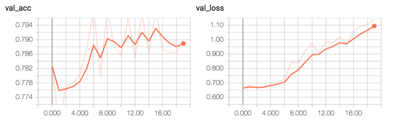 ConvPool-CNN-C验证准确性和验证损失
通过计算测试集上的错误率来评估模型。
def evaluate_error(model):

    pred = model.predict(x_test, batch_size = 32)

    pred = np.argmax(pred, axis=1)

    pred = np.expand_dims(pred, axis=1) # make same shape as y_test

    error = np.sum(np.not_equal(pred, y_test)) / y_test.shape[0]


    return error

evaluate_error(conv_pool_cnn_model)

>>> 0.2414
第二个模型:ALL-CNN-C
下一个CNN,ALL-CNN-C来自同样来自论文。这个模型和上一个非常相似。唯一的区别是用步幅为2的卷积层代替最大池层。再次请注意,Conv2D(10, (1, 1))层之后没有立即使用激活函数。如果在该层之后立即使用了ReLU激活函数,模型将无法训练。
论文:https://arxiv.org/abs/1412.6806v3
def all_cnn(model_input):


    x = Conv2D(96, kernel_size=(3, 3), activation='relu', padding = 'same')(model_input)

    x = Conv2D(96, (3, 3), activation='relu', padding = 'same')(x)

    x = Conv2D(96, (3, 3), activation='relu', padding = 'same', strides = 2)(x)

    x = Conv2D(192, (3, 3), activation='relu', padding = 'same')(x)

    x = Conv2D(192, (3, 3), activation='relu', padding = 'same')(x)

    x = Conv2D(192, (3, 3), activation='relu', padding = 'same', strides = 2)(x)

    x = Conv2D(192, (3, 3), activation='relu', padding = 'same')(x)

    x = Conv2D(192, (1, 1), activation='relu')(x)

    x = Conv2D(10, (1, 1))(x)

    x = GlobalAveragePooling2D()(x)

    x = Activation(activation='softmax')(x)


    model = Model(model_input, x, name='all_cnn')


    return model

all_cnn_model = all_cnn(model_input)

_ = compile_and_train(all_cnn_model, num_epochs=20)
该模型的验证准确性约75%。
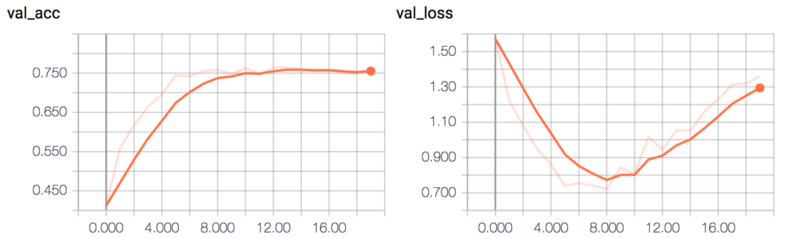 ALL-CNN-C验证的准确性和损失
两个模型非常相似,所以错误率并没有太大的差别。
evaluate_error(all_cnn_model)
>>> 0.26090000000000002
第三个模型:Network In Network CNN
第三个CNN是Network in Network CNN。这个CNN来自这个介绍全局池化层的论文中。它比以前的两个模型更小,因此训练要快得多。同样先不使用激活函数!
论文:https://arxiv.org/abs/1312.4400
我在这里使用1×1内核的卷积层,而不再使用多层感知器内的多层感知器卷积层。通过这种方式可以减少要优化的参数,训练速度更快,并且可以获得更好的结果(使用全连接层时,验证准确性从未高于过50%)。论文中认为,多层感知器网络层的应用功能等价于在常规的卷积层上的cccp层(cascaded cross channel parametric pooling),而后者又等价于具有1x1卷积核的卷积层(如果此处我的解释不正确,请纠正我)。
def nin_cnn(model_input):


    #mlpconv block 1

    x = Conv2D(32, (5, 5), activation='relu',padding='valid')(model_input)

    x = Conv2D(32, (1, 1), activation='relu')(x)

    x = Conv2D(32, (1, 1), activation='relu')(x)

    x = MaxPooling2D((2, 2))(x)

    x = Dropout(0.5)(x)


    #mlpconv block2

    x = Conv2D(64, (3, 3), activation='relu',padding='valid')(x)

    x = Conv2D(64, (1, 1), activation='relu')(x)

    x = Conv2D(64, (1, 1), activation='relu')(x)

    x = MaxPooling2D((2, 2))(x)

    x = Dropout(0.5)(x)


    #mlpconv block3

    x = Conv2D(128, (3, 3), activation='relu',padding='valid')(x)

    x = Conv2D(32, (1, 1), activation='relu')(x)

    x = Conv2D(10, (1, 1))(x)


    x = GlobalAveragePooling2D()(x)

    x = Activation(activation='softmax')(x)


    model = Model(model_input, x, name='nin_cnn')


    return model

nin_cnn_model = nin_cnn(model_input)
这个模型的训练速度要快得多,在我的机器上每次训练要快15秒。
_ = compile_and_train(nin_cnn_model,num_epochs = 20)
该模型达到约65%的验证准确性。
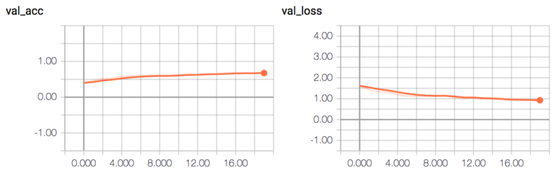 NIN-CNN验证的准确性和损失
因为这个模型比其他两个模型要简单,所以错误率会高一些。
evaluate_error(nin_cnn_model)
>>> 0.31640000000000001
三个模型集成
现在我们将三个模型将被合并到一个集成模型里。
在这里,所有三个模型被重新实例化,并加载已保存的最好权重。
conv_pool_cnn_model = conv_pool_cnn(model_input)

all_cnn_model = all_cnn(model_input)

nin_cnn_model = nin_cnn(model_input)


conv_pool_cnn_model.load_weights('weights / conv_pool_cnn.29-0.10.hdf5')

all_cnn_model.load_weights('weights / all_cnn.30-0.08.hdf5')

nin_cnn_model.load_weights('weights / nin_cnn.30-0.93.hdf5')


models = [conv_pool_cnn_model,all_cnn_model,nin_cnn_model]
集成模型定义非常简单。它使用与以前的所有模型之间共享的相同输入层。在最后一层,集成计算三个模型输出的平均值通过使用Average()合并层。
def ensemble(models, model_input):


    outputs = [model.outputs[0] for model in models]

    y = Average()(outputs)


    model = Model(model_input, y, name='ensemble')


    return model

ensemble_model = ensemble(models, model_input)
和我们的预期一样,集成模型的错误率比任何一个单一的模型都要低。
evaluate_error(ensemble_model)
>>> 0.2049
我们也可以检查由2个模型组成的集成模型的性能。我们发现任意两个模型的集成都比单个模型的错误率更低。
pair_A = [conv_pool_cnn_model, all_cnn_model]

pair_B = [conv_pool_cnn_model, nin_cnn_model]

pair_C = [all_cnn_model, nin_cnn_model]

pair_A_ensemble_model = ensemble(pair_A, model_input)

evaluate_error(pair_A_ensemble_model)
>>> 0.21199999999999999
pair_B_ensemble_model = ensemble(pair_B, model_input)

evaluate_error(pair_B_ensemble_model)
>>> 0.22819999999999999
pair_C_ensemble_model = ensemble(pair_C, model_input)

evaluate_error(pair_C_ensemble_model)
>>> 0.2447
结论
重申介绍中所说的话:每一种模型都有自己的劣势的地方。而集成原因是,通过堆叠不同的模型来表示对数据的不同假设,我们可以通过建立集成在模型的假设空间之外找到一个更好的假设。
通过使用一个非常简单的集成,就实现了,比大多数情况下使用单个模型更低的错误率。这证明了集成很有效果。
当然,在使用机器学习任务的时候要记住结合实际考虑。由于集成意味着将多个模型堆叠在一起,这同样也意味着输入数据需要在每个模型中都要前向传播。这增加了执行所需的计算量,从而增加了评估(或预测)的时间。如果你只是为了研究或比赛,这个时间的增加可能并不重要。但是,在设计商业产品时,这是一个非常关键的因素。另一个考虑因素是如果最终模型的尺寸太大,也可能在商用产品中的使用受到限制。
网页版:https://lawnboymax.github.io/portfolio/keras_ensemble/cnn_ensembling.html