机器学习项目：使用Python进行零售价格推荐

2018年08月08日由 yuxiangyu 发表 981228 0

日本最大的社区购物应用Mercari遇到了一个问题。他们希望向卖家提供定价建议，但这很难，因为他们的卖家能够在Mercari上放置任何东西。

在这个机器学习项目中，我们将建立一个自动建议正确的产品价格的模型。我们提供以下信息：

train_id - 列表的ID

name - 列表的标题

item_condition_id - 卖方提供商品的情况

category_name - 种类的列表

brand_name - 品牌名称

price - 该商品的售价。也就是我们预测的目标变量

shipping - 如果运费由卖方支付，买方支付0

item_description - 商品的完整描述

EDA

数据集可以从Kaggle下载（文末链接）。为了验证结果，我只需要train.tsv。让我们开始吧！

import gc

import time

import numpy as np

import pandas as pd

import matplotlib.pyplot as plt

import seaborn as sns

from scipy.sparse import csr_matrix, hstack

from sklearn.feature_extraction.text import CountVectorizer, TfidfVectorizer

from sklearn.preprocessing import LabelBinarizer

from sklearn.model_selection import train_test_split, cross_val_score

from sklearn.metrics import mean_squared_error

import lightgbm as lgb

df = pd.read_csv('train.tsv', sep = '\t')

随机将数据拆分为训练集和测试集。我们只对EDA使用训练集。

msk = np.random.rand(len(df)) < 0.8

train = df[msk]

test = df[~msk]

train.shape, test.shape

((1185866, 8), (296669, 8))

train.head（）

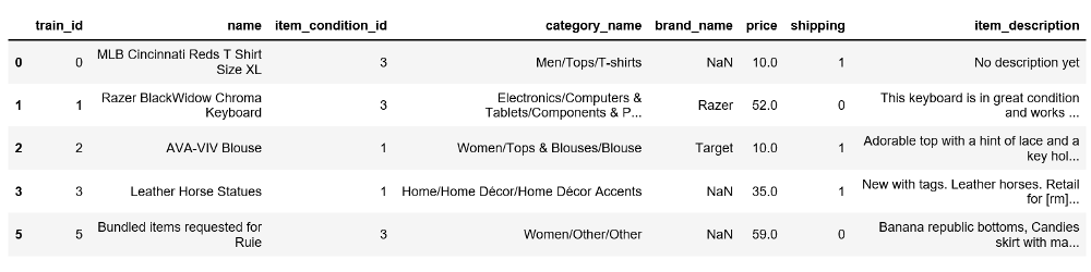
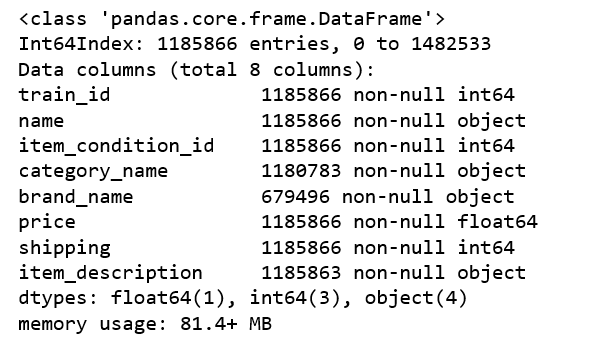
train.info（）

价格

train.price.describe（）

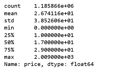
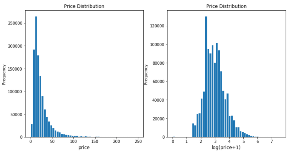
物品价格总体左倾（left skewed），绝大多数物品售价10-20。然而，最昂贵的商品定价在2009。所以我们会对价格进行对数变换。

plt.subplot（1,2,1）

（train ['price']）。plot.hist（bins = 50，figsize =（12,6），edgecolor ='white'，range = [0,250]）

plt .xlabel（'price'，fontsize = 12）

plt.title（'Price Distribution'，fontsize = 12）

plt.subplot（1,2,2）

np.log（train ['price'] + 1）.plot.hist（bins = 50，figsize =（12,6），edgecolor ='white'）

plt.xlabel（ 'log（price + 1）'，fontsize = 12）

plt.title（'Price Distribution'，fontsize = 12）

运费

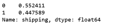
超过55％的物品运费由买家支付。

train ['shipping']。value_counts（）/ len（train）

运费如何与价格相关？

shipping_fee_by_buyer = train.loc[df['shipping'] == 0, 'price']

shipping_fee_by_seller = train.loc[df['shipping'] == 1, 'price']

fig, ax = plt.subplots(figsize=(18,8))

ax.hist(shipping_fee_by_seller, color='#8CB4E1', alpha=1.0, bins=50, range = [0, 100],

       label='Price when Seller pays Shipping')

ax.hist(shipping_fee_by_buyer, color='#007D00', alpha=0.7, bins=50, range = [0, 100],

       label='Price when Buyer pays Shipping')

plt.xlabel('price', fontsize=12)

plt.ylabel('frequency', fontsize=12)

plt.title('Price Distribution by Shipping Type', fontsize=15)

plt.tick_params(labelsize=12)

plt.legend()

plt.show()

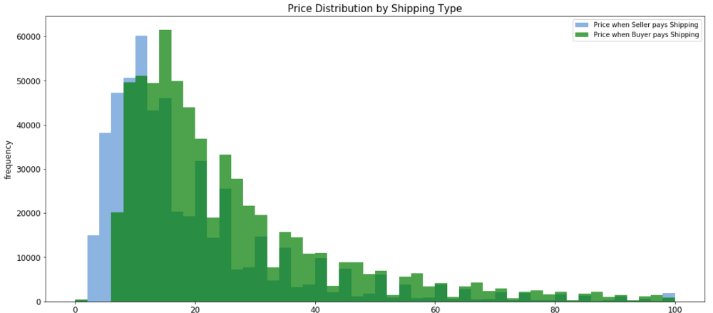
print('The average price is {}'.format(round(shipping_fee_by_seller.mean(), 2)), 'if seller pays shipping');

print('The average price is {}'.format(round(shipping_fee_by_buyer.mean(), 2)), 'if buyer pays shipping')

如果卖家支付运费，平均价格为22.58

如果买家支付运费，平均价格为30.11

我们对价格进行对数转换后再次进行比较。

fig, ax = plt.subplots(figsize=(18,8))

ax.hist(np.log(shipping_fee_by_seller+1), color='#8CB4E1', alpha=1.0, bins=50,

       label='Price when Seller pays Shipping')

ax.hist(np.log(shipping_fee_by_buyer+1), color='#007D00', alpha=0.7, bins=50,

       label='Price when Buyer pays Shipping')

plt.xlabel('log(price+1)', fontsize=12)

plt.ylabel('frequency', fontsize=12)

plt.title('Price Distribution by Shipping Type', fontsize=15)

plt.tick_params(labelsize=12)

plt.legend()

plt.show()

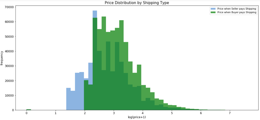
当买家支付运费时，平均价格显然会更高。

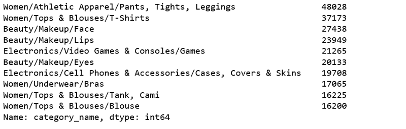
种类名称

print('There are', train['category_name'].nunique(), 'unique values in category name column')

种类名称列中有1265个唯一值

十大最常见的种类名称：

train['category_name'].value_counts()[:10]

商品情况与价格

sns.boxplot（x ='item_condition_id'，y = np.log（train ['price'] + 1），data = train，palette = sns.color_palette（'RdBu'，5））

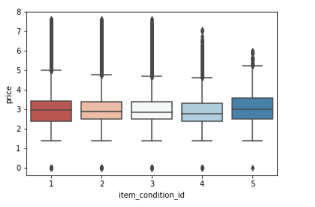
每个商品状态id的平均价格都不大一样。

经过以上的探索性数据分析，我决定使用所有的特征来构建我们的模型。

LightGBM

LightGBM是一个使用基于树的学习算法的梯度提升框架。具有它被设计成分布式且高效性的，它的优点包括：

更快的训练速度和更高的效率

更低的内存使用率

更高的准确性

支持并行和GPU学习

能够处理大规模数据

因此，我们要尝试一下。

常规设置：

NUM_BRANDS = 4000 

NUM_CATEGORIES = 1000 

NAME_MIN_DF = 10 

MAX_FEATURES_ITEM_DESCRIPTION = 50000

我们必须修复的列中缺失值：

print('There are %d items that do not have a category name.' %train['category_name'].isnull().sum())

有5083个商品没有种类名称。

print('There are %d items that do not have a brand name.' %train['brand_name'].isnull().sum())

有506370个商品没有品牌名称。

print('There are %d items that do not have a description.' %train['item_description'].isnull().sum())

有3个商品没有描述。

LightGBM的助手函数：

def handle_missing_inplace(dataset): 

    dataset['category_name'].fillna(value='missing', inplace=True) 

    dataset['brand_name'].fillna(value='missing', inplace=True) 

    dataset['item_description'].replace('No description yet,''missing', inplace=True) 

    dataset['item_description'].fillna(value='missing', inplace=True)

def cutting(dataset):

    pop_brand = dataset['brand_name'].value_counts().loc[lambda x: x.index != 'missing'].index[:NUM_BRANDS]

    dataset.loc[~dataset['brand_name'].isin(pop_brand), 'brand_name'] = 'missing'

    pop_category = dataset['category_name'].value_counts().loc[lambda x: x.index != 'missing'].index[:NUM_CATEGORIES]

def to_categorical(dataset):

    dataset['category_name'] = dataset['category_name'].astype('category')

    dataset['brand_name'] = dataset['brand_name'].astype('category')

    dataset['item_condition_id'] = dataset['item_condition_id'].astype('category')

删除price = 0的行

df = pd.read_csv（'train.tsv'，sep ='\ t'）

msk = np.random.rand（len（df））<0.8 

train = df [msk] 

test = df [~msk] 

test_new = test .drop（'price'，axis = 1）

y_test = np.log1p（test [“price”]）

train = train [train.price！= 0] .reset_index（drop = True）

合并训练和新的测试数据。

nrow_train = train.shape [0] 

y = np.log1p（train [“price”]）

merge：pd.DataFrame = pd.concat（[train，test_new]）

训练准备

handle_missing_inplace（merge）

cutting（merge）

to_categorical（merge）

计算矢量化名称和种类名称的列。

cv = CountVectorizer（min_df = NAME_MIN_DF）

X_name = cv.fit_transform（merge ['name']）

cv = CountVectorizer（）

X_category = cv.fit_transform（merge ['category_name']）

TF-IDF Vectorize item_description列。

tv = TfidfVectorizer（max_features = MAX_FEATURES_ITEM_DESCRIPTION，ngram_range =（1,3），stop_words ='english'）

X_description = tv.fit_transform（merge ['item_description']）

标签二值化brand_name列。

lb = LabelBinarizer（sparse_output = True）

X_brand = lb.fit_transform（merge ['brand_name']）

为item_condition_id和运费列创建虚拟变量。

X_dummies = csr_matrix（pd.get_dummies（merge [['item_condition_id'，'shipping']]，sparse = True）.values）

创建稀疏合并。

sparse_merge = hstack（（X_dummies，X_description，X_brand，X_category，X_name））。tocsr（）

删除文档频率<= 1的特征。

mask = np.array（np.clip（sparse_merge.getnnz（axis = 0） - 

1,0,1 ），dtype = bool）sparse_merge = sparse_merge [：，mask]

从稀疏合并中分离出训练和测试数据。

X = sparse_merge [：nrow_train] 

X_test = sparse_merge [nrow_train：]

为lightgbm创建数据集。

train_X = lgb.Dataset（X，label = y）

将我们的参数指定为dict。

params = { 

        'learning_rate'：0.75，

        'application'：'regression'，

        'max_depth'：3，

        'num_leaves'：100，

        'verbosity'： -  1，

        'metric'：'RMSE'，

    }

当我们处理回归问题时，使用“regression”作为应用程序。

使用“RMSE”作为度量，因为这是一个回归问题。

“num_leaves”= 100，因为我们的数据相对较大。

使用“max_depth”以避免过拟合。

使用“verbosity”来控制LightGBM的冗余度（<0：致命）。

“learning_rate”确定每棵树对最终结果的影响。

训练开始

训练模型需要参数列表和数据集。训练需要一段时间。

gbm = lgb.train（params，train_set = train_X，num_boost_round = 3200，verbose_eval = 100）

预测

y_pred = gbm.predict（X_test，num_iteration = gbm.best_iteration）

评估

from sklearn.metrics import mean_squared_error

print('The rmse of prediction is:', mean_squared_error(y_test, y_pred) ** 0.5)

预测的rmse是：0.46164222941613137

Kaggle：https://www.kaggle.com/tunguz/more-effective-ridge-lgbm-script-lb-0-44823

Github：https://github.com/susanli2016/Machine-Learning-with-Python/blob/master/Mercari%20Price%20Suggestion%20Lightgbm.ipynb

数据集：https://www.kaggle.com/saitosean/mercari

标签：

Python 学习开源项目

0 评论

欢迎关注ATYUN官方公众号

商务合作及内容投稿请联系邮箱:bd@atyun.com

上一篇不需要大把的GPU如何赢得Kaggle比赛？fast.ai给出的十个技巧

下一篇机器学习实例：文本挖掘和情感分析的基础示例

评论登录

要发表评论，您必须先登录。

jonatasgrosman/wav2vec2-large-xlsr-53-english facebook/dino-vitb16 bert-base-uncased xlm-roberta-large xlm-roberta-base gpt2 microsoft/resnet-50 facebook/dino-vits8

Sam Altman离职事件时间线