机器学习实例:文本挖掘和情感分析的基础示例

经过研究表明,在旅行者的决策过程中,TripAdvisor(猫途鹰,全球旅游点评网)正变得越来越重要。然而,了解TripAdvisor评分与数千个评论文本中的每一个的细微差别是很有挑战性的。为了更彻底地了解酒店客人的评论是否会影响酒店的加班表现,我从TripAdvisor截取了一家酒店 - 希尔顿夏威夷度假村(Hilton Hawaiian Village)的所有英语评论 (Web抓取的细节和Python代码在文末)。
加载库
library(dplyr)

library(readr)

library(lubridate)

library(ggplot2)

library(tidytext)

library(tidyverse)

library(stringr)

library(tidyr)

library(scales)

library(broom)

library(purrr)

library(widyr)

library(igraph)

library(ggraph)

library(SnowballC)

library(wordcloud)

library(reshape2)

theme_set(theme_minimal())
数据
df <- read_csv("Hilton_Hawaiian_Village_Waikiki_Beach_Resort-Honolulu_Oahu_Hawaii__en.csv")

df <- df[complete.cases(df), ]

df$review_date <- as.Date(df$review_date, format = "%d-%B-%y")

dim(df); min(df$review_date); max(df$review_date)
在TripAdvisor上希尔顿夏威夷度假村共有13,701条评论,评论日期范围是2002-03-21到2018-08-02。
df %>%

  count(Week = round_date(review_date, "week")) %>%

  ggplot(aes(Week, n)) +

  geom_line() +

  ggtitle('The Number of Reviews Per Week')
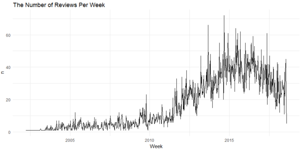
2014年底收到的每周评论数量最多。该酒店在那一周收到了70多条评论。
评论文本的文本挖掘
df <- tibble::rowid_to_column(df, "ID")

df <- df %>%

  mutate(review_date = as.POSIXct(review_date, origin = "1970-01-01"),month = round_date(review_date, "month"))

review_words <- df %>%

  distinct(review_body, .keep_all = TRUE) %>%

  unnest_tokens(word, review_body, drop = FALSE) %>%

  distinct(ID, word, .keep_all = TRUE) %>%

  anti_join(stop_words, by = "word") %>%

  filter(str_detect(word, "[^\\d]")) %>%

  group_by(word) %>%

  mutate(word_total = n()) %>%

  ungroup()

word_counts <- review_words %>%

  count(word, sort = TRUE)

word_counts %>%

  head(25) %>%

  mutate(word = reorder(word, n)) %>%

  ggplot(aes(word, n)) +

  geom_col(fill = "lightblue") +

  scale_y_continuous(labels = comma_format()) +

  coord_flip() +

  labs(title = "Most common words in review text 2002 to date",

       subtitle = "Among 13,701 reviews; stop words removed",

       y = "# of uses")
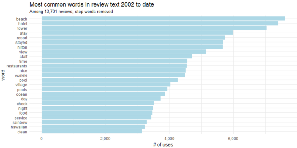
我们肯定可以做得更好一些,将“stay ”和“stayed ”,“pool”和“pools ”合起来。这被称为词干,词干是将变形(或有时是衍生)的词语变回到词干,基词或根词格式的过程。
word_counts %>%
head(25) %>%
mutate(word = wordStem(word)) %>%
mutate(word = reorder(word, n)) %>%
ggplot(aes(word, n)) +
geom_col(fill = "lightblue") +
scale_y_continuous(labels = comma_format()) +
coord_flip() +
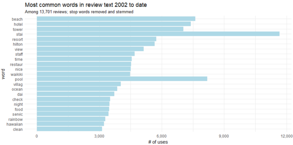
labs(title = "Most common words in review text 2002 to date",
subtitle = "Among 13,701 reviews; stop words removed and stemmed",
y = "# of uses")
bigram
我们经常想要了解评论中单词之间的关系。在评论文本中,有哪些常见的单词序列?给定一些单词,哪些单词最有可能跟随在这个单词后面?哪些词关联最紧密?因此,许多有趣的文本分析都是基于这种关联。当我们检查两个连续单词的对时,它被称为“bigram”(二元语法)。
那么,这家酒店的评论中最常见的bigram评论是什么?
review_bigrams <- df %>%

  unnest_tokens(bigram, review_body, token = "ngrams", n = 2)

bigrams_separated <- review_bigrams %>%

  separate(bigram, c("word1", "word2"), sep = " ")

bigrams_filtered <- bigrams_separated %>%

  filter(!word1 %in% stop_words$word) %>%

  filter(!word2 %in% stop_words$word)

bigram_counts <- bigrams_filtered %>%

  count(word1, word2, sort = TRUE)

bigrams_united <- bigrams_filtered %>%

  unite(bigram, word1, word2, sep = " ")

bigrams_united %>%

  count(bigram, sort = TRUE)
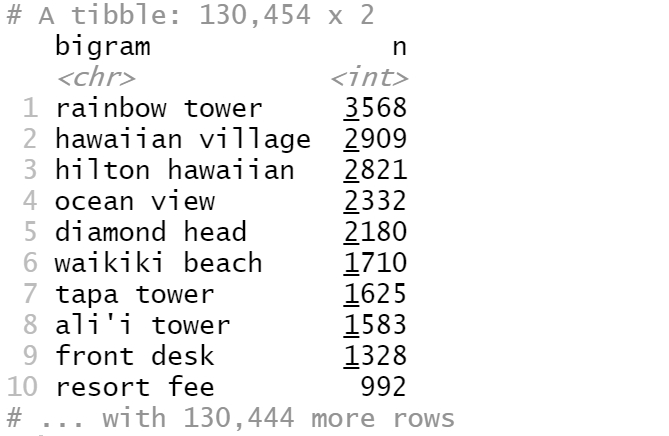
最常见的bigram是“rainbow tower”,其次是“hawaiian village”。
我们可以在单词网络中可视化bigram:
review_subject <- df %>%

  unnest_tokens(word, review_body) %>%

  anti_join(stop_words)

my_stopwords <- data_frame(word = c(as.character(1:10)))

review_subject <- review_subject %>%

  anti_join(my_stopwords)

title_word_pairs <- review_subject %>%

  pairwise_count(word, ID, sort = TRUE, upper = FALSE)

set.seed(1234)

title_word_pairs %>%

  filter(n >= 1000) %>%

  graph_from_data_frame() %>%

  ggraph(layout = "fr") +

  geom_edge_link(aes(edge_alpha = n, edge_width = n), edge_colour = "cyan4") +

  geom_node_point(size = 5) +

  geom_node_text(aes(label = name), repel = TRUE,

                 point.padding = unit(0.2, "lines")) +

  ggtitle('Word network in TripAdvisor reviews')

  theme_void()
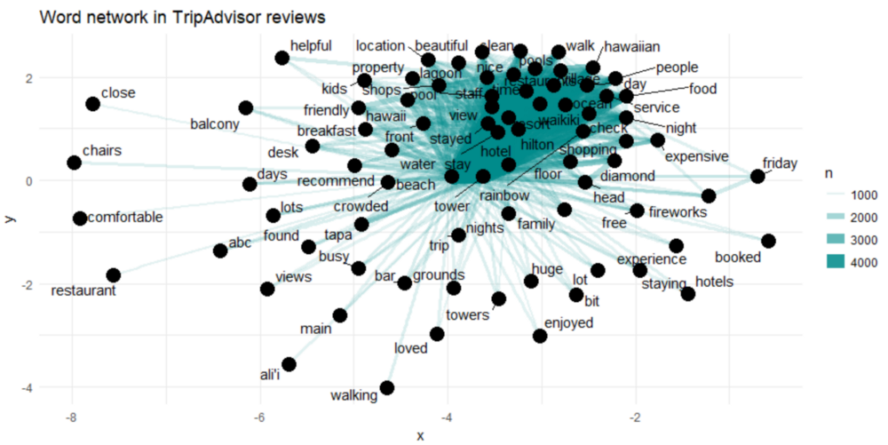
上面显示了TripAdvisor评论中常见的bigram组合,显示了至少出现了1000次且不是停用词的单词。
网络图显示了前几个词(“hawaiian ”,“village ”,“ocean ”和“view ”)之间的紧密联系。然而,我们在网络中并没有看到清晰的聚类结构。
Trigram
Bigram有时是不够的,让我们看看希尔顿夏威夷度假村在TripAdvisor评论中最常见的trigram(三元语法)?
review_trigrams <- df %>%

  unnest_tokens(trigram, review_body, token = "ngrams", n = 3)


trigrams_separated <- review_trigrams %>%

  separate(trigram, c("word1", "word2", "word3"), sep = " ")


trigrams_filtered <- trigrams_separated %>%

  filter(!word1 %in% stop_words$word) %>%

  filter(!word2 %in% stop_words$word) %>%

  filter(!word3 %in% stop_words$word)


trigram_counts <- trigrams_filtered %>%

  count(word1, word2, word3, sort = TRUE)


trigrams_united <- trigrams_filtered %>%

  unite(trigram, word1, word2, word3, sep = " ")


trigrams_united %>%

  count(trigram, sort = TRUE)
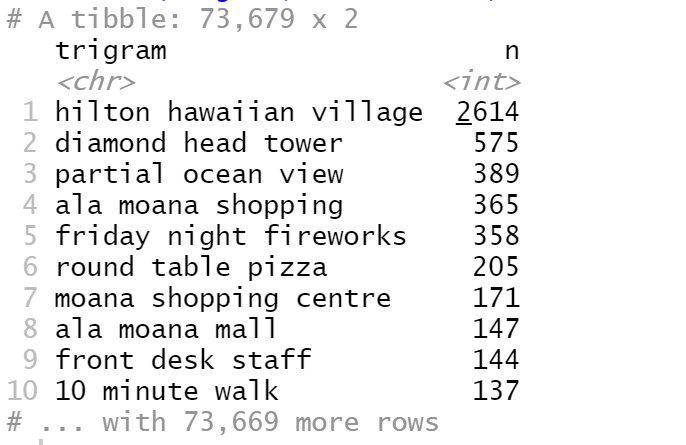
最常见的trigram 是“hilton hawaiian village”,其次是“hilton hawaiian village”,依此类推。
评论中的重要的词汇趋势
随着时间的推移,哪些词语和话题变得更频繁(或者更频繁)了?这些可以让我们了解酒店不断变化的生态系统,例如服务,翻新,问题解决,让我们预测哪些话题的关联词将继续增长。
我们需要了解的问题是:在TripAdvisor评论中,随着时间的推移,哪些词的频率在增加?
reviews_per_month <- df %>%

  group_by(month) %>%

  summarize(month_total = n())

word_month_counts <- review_words %>%

  filter(word_total >= 1000) %>%

  count(word, month) %>%

  complete(word, month, fill = list(n = 0)) %>%

  inner_join(reviews_per_month, by = "month") %>%

  mutate(percent = n / month_total) %>%

  mutate(year = year(month) + yday(month) / 365)

mod <- ~ glm(cbind(n, month_total - n) ~ year, ., family = "binomial")

slopes <- word_month_counts %>%

  nest(-word) %>%

  mutate(model = map(data, mod)) %>%

  unnest(map(model, tidy)) %>%

  filter(term == "year") %>%

  arrange(desc(estimate))

slopes %>%

  head(9) %>%

  inner_join(word_month_counts, by = "word") %>%

  mutate(word = reorder(word, -estimate)) %>%

  ggplot(aes(month, n / month_total, color = word)) +

  geom_line(show.legend = FALSE) +

  scale_y_continuous(labels = percent_format()) +

  facet_wrap(~ word, scales = "free_y") +

  expand_limits(y = 0) +

  labs(x = "Year",

       y = "Percentage of reviews containing this word",

       title = "9 fastest growing words in TripAdvisor reviews",

       subtitle = "Judged by growth rate over 15 years")
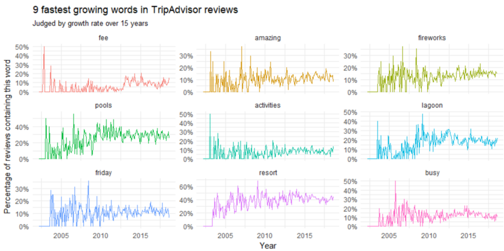
在2010年之前,我们可以看到关于“friday fireworks”和“lagoon”的讨论高峰。像“resort fee”和“busy”这样的词在2005年之前增长最快。
在评论中,哪些词的频率在下降?
word_month_counts %>%

  filter(word %in% c("service", "food")) %>%

  ggplot(aes(month, n / month_total, color = word)) +

  geom_line(size = 1, alpha = .8) +

  scale_y_continuous(labels = percent_format()) +

  expand_limits(y = 0) +

  labs(x = "Year",

       y = "Percentage of reviews containing this term", title = "service vs food in terms of reviewers interest")
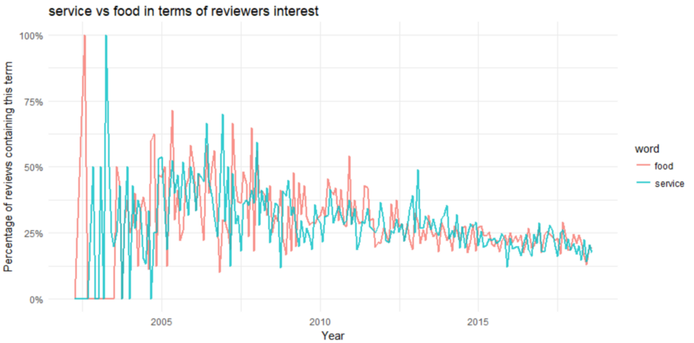
服务和食品都是2010年之前的主要话题。关于服务和食品的讨论在2003年左右的数据开始时达到顶峰,在2005年之后一直呈下降趋势,偶尔出现高峰。
情绪分析
情感分析广泛应用于客户反馈,需要分析的有:评论和调查结果,在线和社交媒体。它适用于从营销到客户服务以及临床医学的各种应用。
在我们的案例中,我们的目的是确定评论者(即酒店客人)对他过去对酒店的体验的看法。这种可能是判断或评价。
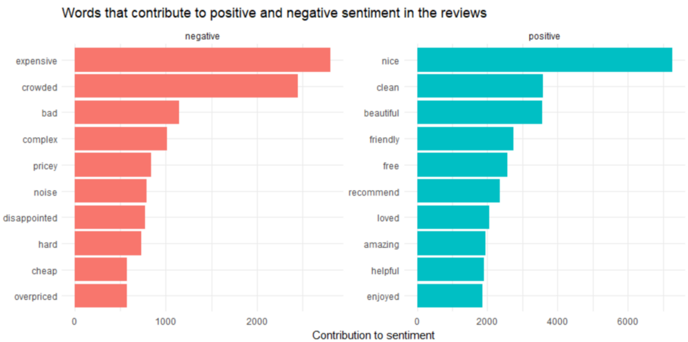
评论中最常见的正面和负面词汇。
reviews <- df %>%

  filter(!is.na(review_body)) %>%

  select(ID, review_body) %>%

  group_by(row_number()) %>%

  ungroup()

tidy_reviews <- reviews %>%

  unnest_tokens(word, review_body)

tidy_reviews <- tidy_reviews %>%

  anti_join(stop_words)


bing_word_counts <- tidy_reviews %>%

  inner_join(get_sentiments("bing")) %>%

  count(word, sentiment, sort = TRUE) %>%

  ungroup()


bing_word_counts %>%

  group_by(sentiment) %>%

  top_n(10) %>%

  ungroup() %>%

  mutate(word = reorder(word, n)) %>%

  ggplot(aes(word, n, fill = sentiment)) +

  geom_col(show.legend = FALSE) +

  facet_wrap(~sentiment, scales = "free") +

  labs(y = "Contribution to sentiment", x = NULL) +

  coord_flip() +

  ggtitle('Words that contribute to positive and negative sentiment in the reviews')
让我们试试另一个情绪库,看看结果是否相同。
contributions <- tidy_reviews %>%

  inner_join(get_sentiments("afinn"), by = "word") %>%

  group_by(word) %>%

  summarize(occurences = n(),

            contribution = sum(score))

contributions %>%

  top_n(25, abs(contribution)) %>%

  mutate(word = reorder(word, contribution)) %>%

  ggplot(aes(word, contribution, fill = contribution > 0)) +

  ggtitle('Words with the greatest contributions to positive/negative

          sentiment in reviews') +

  geom_col(show.legend = FALSE) +

  coord_flip()
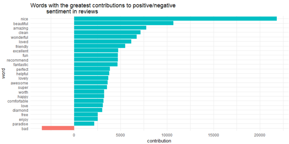
有趣的是,“diamond ”(diamond head)被归类为积极的情绪。
这里有一个可能出现的问题,例如,“clean”,在不通的上下文,如前面带有“not”,则会产生负面情绪。事实上,在大多数unigram(一元模型)会有这个否定的问题。所以我们需要进行下一步:
使用Bigrams在情感分析中提供语境
我们想知道单词前面有“not”这样的单词的频率。
bigrams_separated %>%

  filter(word1 == "not") %>%

  count(word1, word2, sort = TRUE)
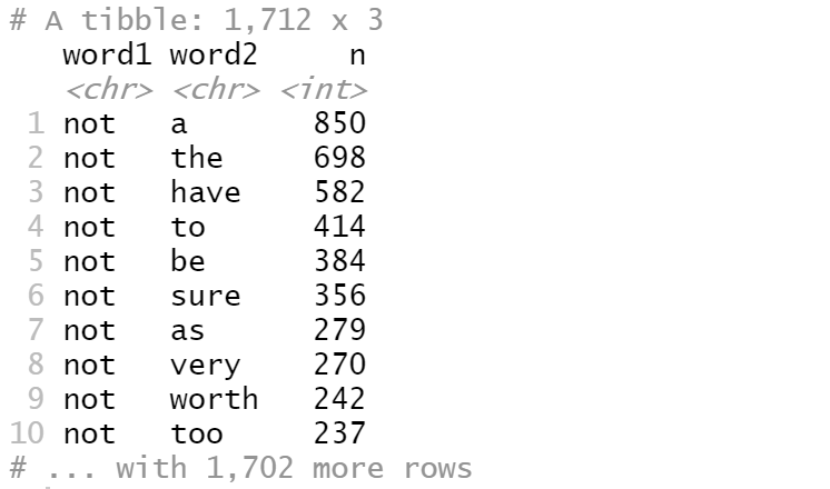
数据中有850次单词“a”前面有单词“not”,而698次单词“the”前面单词“not”。但这些信息没有意义。
AFINN <- get_sentiments("afinn")

not_words <- bigrams_separated %>%

  filter(word1 == "not") %>%

  inner_join(AFINN, by = c(word2 = "word")) %>%

  count(word2, score, sort = TRUE) %>%

  ungroup()


not_words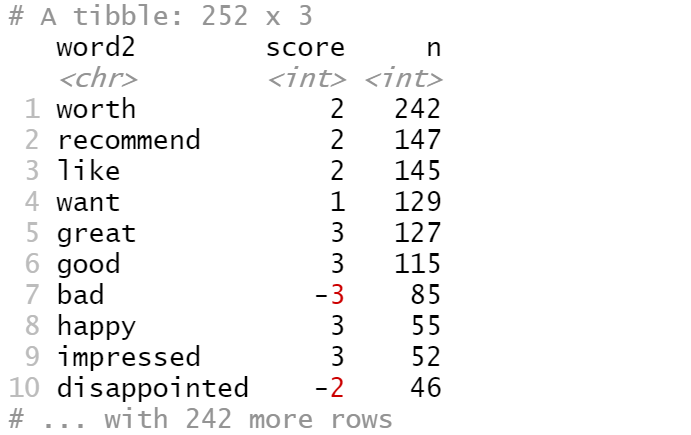
这告诉我们,在数据中,跟随“not”的最常见的情感关联词是“worth”,而跟随“not”的第二个常见情感关联词是“recommend”,这通常得分为2分。
那么,在我们的数据中,哪些词在错误的方向上做了最大的“贡献”呢?
not_words %>%

  mutate(contribution = n * score) %>%

  arrange(desc(abs(contribution))) %>%

  head(20) %>%

  mutate(word2 = reorder(word2, contribution)) %>%

  ggplot(aes(word2, n * score, fill = n * score > 0)) +

  geom_col(show.legend = FALSE) +

  xlab("Words preceded by \"not\"") +

  ylab("Sentiment score * number of occurrences") +

  ggtitle('The 20 words preceded by "not" that had the greatest contribution to

          sentiment scores, positive or negative direction') +

  coord_flip()
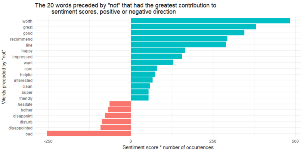
“not worth”,“not great”,“not good”,“not recommend”和“not like”的最大的错误识别原因,这使得文本看起来比实际上更积极。
除了“not”之外,还有其他词语否定后续词语,例如“no”,“never”和“without”。
negation_words <- c("not", "no", "never", "without")


negated_words <- bigrams_separated %>%

  filter(word1 %in% negation_words) %>%

  inner_join(AFINN, by = c(word2 = "word")) %>%

  count(word1, word2, score, sort = TRUE) %>%

  ungroup()


negated_words %>%

  mutate(contribution = n * score,

         word2 = reorder(paste(word2, word1, sep = "__"), contribution)) %>%

  group_by(word1) %>%

  top_n(12, abs(contribution)) %>%

  ggplot(aes(word2, contribution, fill = n * score > 0)) +

  geom_col(show.legend = FALSE) +

  facet_wrap(~ word1, scales = "free") +

  scale_x_discrete(labels = function(x) gsub("__.+$", "", x)) +

  xlab("Words preceded by negation term") +

  ylab("Sentiment score * # of occurrences") +

  ggtitle('The most common positive or negative words to follow negations

          such as "no", "not", "never" and "without"') +

  coord_flip()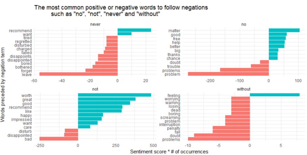
看起来把一个词误认为是正面情绪的最大来源是“not worth/great/good/recommend”,而错误分类的负面情绪的最大来源是“not bad”和“no problem”。
最后,让我们找出最正面和最负面的评论。
sentiment_messages <- tidy_reviews %>%

  inner_join(get_sentiments("afinn"), by = "word") %>%

  group_by(ID) %>%

  summarize(sentiment = mean(score),

            words = n()) %>%

  ungroup() %>%

  filter(words >= 5)

sentiment_messages %>%

  arrange(desc(sentiment))
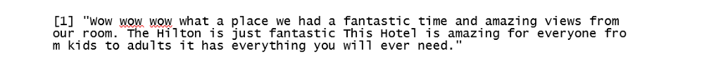
最正面的评论ID是2363:
df [which(df $ ID == 2363),] $ review_body [1]
sentiment_messages %>%

  arrange(sentiment)
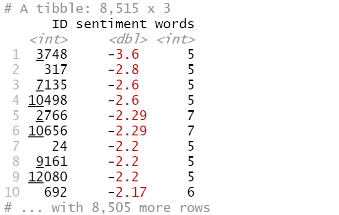
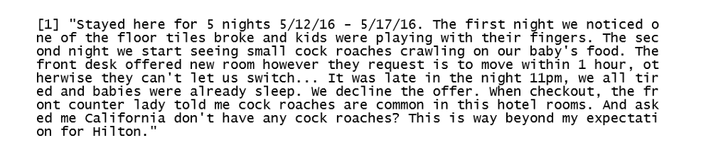
最负面评论的ID为3748:
df [which(df $ ID == 3748),] $ review_body [1]
Github:https://github.com/susanli2016/Data-Analysis-with-R/blob/master/Text%20Mining%20Hilton%20Hawaiian%20Village%20TripAdvisor%20Reviews.Rmd
负责抓取的Python代码:https://github.com/susanli2016/NLP-with-Python/blob/master/Web%20scraping%20Hilton%20Hawaiian%20Village%20TripAdvisor%20Reviews.py