


请先登录您的atyun账户,方可使用该功能

审核通过后即可使用此功能,请耐心等待~


优化算法:到底是数学还是代码?
2017年11月22日 由 yining 发表
875232
0
背景:我的一位同事曾提到,他在面试深度学习相关职位中被问到一些关于优化算法的问题。我决定在本文中就优化算法做一个简短的介绍。
成本函数的最优化算法
目标函数是一种试图将一组参数最小化的函数。在机器学习中,目标函数通常被设定为一种度量,即预测值与实际值的相似程度。通常,我们希望找到一组会导致尽可能小的成本的参数,因为这就意味着你的算法会完成得很好。一个函数的最小成本可能就是最小值。有时,成本函数可以有多个局部最小值。幸运的是,在非常高维的参数空间中,保护目标函数的充分优化的局部极小值不会经常发生,因为这意味着在过程的早期,每个参数都为凹(concave)。这不是典型的情况,所以我们剩下了很多鞍点(saddle point),而不是真正的最小值。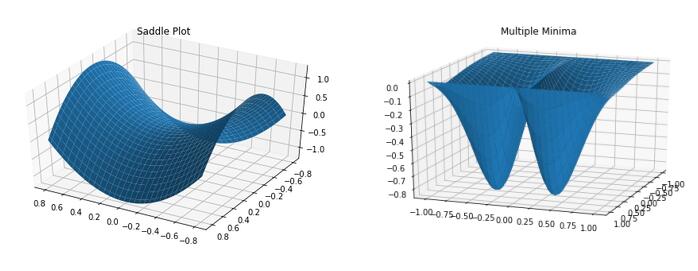
找到导致最小值的参数集的算法被称为优化算法。随着算法复杂度的增加,我们会发现它们能够更有效地达到最小值。在这篇文章中,我们将讨论四种优化算法,包括:
- 随机梯度下降算法(SGD)
- Momentum算法
- RMSProp算法
- Adam算法
随机梯度下降算法
在随机梯度下降算法中,你很可能会遇到这样的方程: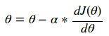
θ(theta)是你想要找到使J最小化的最优值。J在这里这被称为目标函数。最后我们得到了一个被称为α(alpha)的学习速率。反复评估这个函数直到你达到预期的成本。
这是什么意思?设想一下,你坐在山顶上的雪橇上,望着另一座山。如果你滑下山坡,直到你最终到达底部之前,你会一直向下移动。如果第一座山足够陡峭,你可能会开始沿着另一座山向上爬。在这个类比中,你可以认为:
θ:作为山的位置
 :作为角度θ大小的陡坡
α:作为
高学习率意味着低摩擦(friction),因此雪橇会像在冰上一样,沿着山坡急速下降。低学习率意味着高摩擦,所以雪橇就像在地毯上一样,挣扎着从山坡上往下滑。我们如何用上面的方程来模拟这种效果呢?
随机梯度下降算法:
1.初始化参数(θ,学习速率)
2.计算每个角度θ的梯度
3.更新参数
4.重复步骤2和步骤3,直到成本稳定
让我们来以一个简单的例子来看看它是如何工作的!
这里我们看到了一个目标函数和它的导数(梯度):
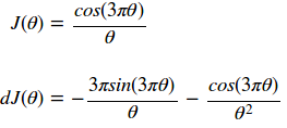
我们可以用下面的代码生成一个函数的图,以代码的形式表示1/30的它的梯度(倾斜度):
import numpy as np


def minimaFunction(theta):

    return np.cos(3*np.pi*theta)/theta


def minimaFunctionDerivative(theta):

    const1 = 3*np.pi

    const2 = const1*theta

    return -(const1*np.sin(const2)/theta)-np.cos(const2)/theta**2


theta = np.arange(.1,2.1,.01)

Jtheta = minimaFunction(theta)

dJtheta = minimaFunctionDerivative(theta)


plt.plot(theta,Jtheta,label = r'$J(\theta)$')

plt.plot(theta,dJtheta/30,label = r'$dJ(\theta)/30$')

plt.legend()

axes = plt.gca()

#axes.set_ylim([-10,10])


plt.ylabel(r'$J(\theta),dJ(\theta)/30$')

plt.xlabel(r'$\theta$')

plt.title(r'$J(\theta),dJ(\theta)/30 $ vs $\theta$')

plt.show()
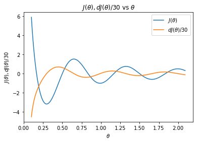
在上面的图中,有两件事十分引人注目。首先,请注意这个成本函数是如何有一些最小值的(大约为2.25、1.0和1.7)。其次,注意到导数在最小值处等于0,在拐点处等于最大的数值。这个特点是我们在随机梯度下降算法中所要利用的。
我们可以在下面的代码中看到上述四个步骤的实现。下面的视频显示了θ的值和每个步长的梯度。
import numpy as np

import matplotlib.pyplot as plt

import matplotlib.animation as animation


def optimize(iterations, oF, dOF,params,learningRate):

    """

    computes the optimal value of params for a given objective function and its derivative

    Arguments:

        - iteratoins - the number of iterations required to optimize the objective function

        - oF - the objective function

        - dOF - the derivative function of the objective function

        - params - the parameters of the function to optimize

        - learningRate - the learning rate

    Return:

        - oParams - the list of optimized parameters at each step of iteration

    """

    oParams = [params]

    #The iteration loop

    for i in range(iterations):

        # Compute the derivative of the parameters

        dParams = dOF(params)

        # Compute the update

        params = params-learningRate*dParams


        # app end the new parameters

        oParams.append(params)


    return np.array(oParams)


def minimaFunction(theta):

    return np.cos(3*np.pi*theta)/theta


def minimaFunctionDerivative(theta):

    const1 = 3*np.pi

    const2 = const1*theta

    return -(const1*np.sin(const2)/theta)-np.cos(const2)/theta**2


theta = .6

iterations=45

learningRate = .0007

optimizedParameters = optimize(iterations,\

                               minimaFunction,\

                               minimaFunctionDerivative,\

                               theta,\

                               learningRate)
这看起来效果很好!你应该注意到,如果θ的初始值较大,那么优化算法将会在另一个局部极小值中出现。然而,正如上面所提到的,在一个极其高维的空间中存在一个糟糕的、真正的最小值的机会是不太可能的,因为它将要求所有的参数同时为凹。
你可能会想,“如果我们的学习速率太大的话,会发生什么?”如果步长太大,那么算法可能永远无法找到下面动画中所示的那种最优情况。监控成本函数,并确保其总体上是否单调递减是十分重要的。如果不是,你就必须降低学习速率。
随机梯度下降算法也适用于多变量参数空间的情况。我们可以把2D的函数画成等值线图。在这里你可以看到随机梯度下降算法在一个不对称的碗形函数上工作。
import numpy as np

import matplotlib.mlab as mlab

import matplotlib.pyplot as plt

import scipy.stats

import matplotlib.animation as animation


def minimaFunction(params):

    #Bivariate Normal function

    X,Y = params


    sigma11,sigma12,mu11,mu12 = (3.0,.5,0.0,0.0)


    Z1 = mlab.bivariate_normal(X, Y, sigma11,sigma12,mu11,mu12)


    Z = Z1


    return -40*Z


def minimaFunctionDerivative(params):

    # Derivative of the bivariate normal function

    X,Y = params


    sigma11,sigma12,mu11,mu12 = (3.0,.5,0.0,0.0)


    dZ1X = -scipy.stats.norm.pdf(X, mu11, sigma11)*(mu11 - X)/sigma11**2

    dZ1Y = -scipy.stats.norm.pdf(Y, mu12, sigma12)*(mu12 - Y)/sigma12**2


    return (dZ1X,dZ1Y)


def optimize(iterations, oF, dOF,params,learningRate,beta):

    """

    computes the optimal value of params for a given objective function and its derivative

    Arguments:

        - iteratoins - the number of iterations required to optimize the objective function

        - oF - the objective function

        - dOF - the derivative function of the objective function

        - params - the parameters of the function to optimize

        - learningRate - the learning rate

- beta - The weighted moving average parameter

    Return:

        - oParams - the list of optimized parameters at each step of iteration

    """

    oParams = [params]

    vdw     = (0.0,0.0)

    #The iteration loop

    for i in range(iterations):

        # Compute the derivative of the parameters

        dParams = dOF(params)


        #SGD in this line Goes through each parameter and applies parameter = parameter -learningrate*dParameter

        params = tuple([par-learningRate*dPar for dPar,par in zip(dParams,params)])


        # append the new parameters

        oParams.append(params)


    return oParams


iterations=100

learningRate = 1

beta = .9

x,y = 4.0,1.0

params = (x,y)

optimizedParameters = optimize(iterations,\

                               minimaFunction,\

                               minimaFunctionDerivative,\

                               params,\

                               learningRate,\

                               beta)
随机梯度下降算法与Momentum算法
通常情况下,我们希望使用非常大的学习速率来快速学习感兴趣的参数。不幸的是,当成本面很窄时,这可能会导致参数不稳定。在前一段视频中,你可以看到y参数方向上的颠簸,以及对最小值的水平方向的缺失。Momentum算法试图通过预测过去的梯度来解决这个问题。通常情况下,随机梯度下降算法和Momentum算法更新参数以下面的方程式表示:
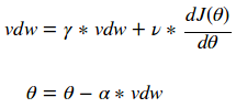
γ(gamma)和ν(nu)值允许用户对dJ(θ)的前一个值和当前值进行加权,以确定θ的新值。人们很普遍地选择γ和ν的值来创建一个指数的加权移动平均,如下所示:
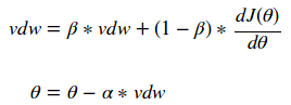
测试参数的一个好的起始点是0.9。选择一个等于1-1/t的β(beta)值,可以让我们更强烈地考虑vdw的最后的t值。这种优化的简单更改可以产生惊人的结果!我们现在可以使用更大的学习速率,并且在一小段时间内集中在解决方案上!
import numpy as np

import matplotlib.mlab as mlab

import matplotlib.pyplot as plt

import scipy.stats

import matplotlib.animation as animation


def minimaFunction(params):

    #Bivariate Normal function

    X,Y = params


    sigma11,sigma12,mu11,mu12 = (3.0,.5,0.0,0.0)


    Z1 = mlab.bivariate_normal(X, Y, sigma11,sigma12,mu11,mu12)


    Z = Z1


    return -40*Z


def minimaFunctionDerivative(params):

    # Derivative of the bivariate normal function

    X,Y = params


    sigma11,sigma12,mu11,mu12 = (3.0,.5,0.0,0.0)


    dZ1X = -scipy.stats.norm.pdf(X, mu11, sigma11)*(mu11 - X)/sigma11**2

    dZ1Y = -scipy.stats.norm.pdf(Y, mu12, sigma12)*(mu12 - Y)/sigma12**2


    return (dZ1X,dZ1Y)


def optimize(iterations, oF, dOF,params,learningRate,beta):

    """

    computes the optimal value of params for a given objective function and its derivative

    Arguments:

        - iteratoins - the number of iterations required to optimize the objective function

        - oF - the objective function

        - dOF - the derivative function of the objective function

        - params - the parameters of the function to optimize

        - learningRate - the learning rate

- beta - The weighted moving average parameter for momentum

    Return:

        - oParams - the list of optimized parameters at each step of iteration

    """

    oParams = [params]

    vdw     = (0.0,0.0)

    #The iteration loop

    for i in range(iterations):

        # Compute the derivative of the parameters

        dParams = dOF(params)


        # Compute the momentum of each gradient vdw = vdw*beta+(1.0+beta)*dPar

        vdw = tuple([vDW*beta+(1.0-beta)*dPar for dPar,vDW in zip(dParams,vdw)])


        #SGD in this line Goes through each parameter and applies parameter = parameter -learningrate*dParameter

        params = tuple([par-learningRate*dPar for dPar,par in zip(vdw,params)])


        # append the new parameters

        oParams.append(params)


    return oParams


iterations=100

learningRate = 5.3

beta = .9

x,y = 4.0,1.0

params = (x,y)

optimizedParameters = optimize(iterations,\

                               minimaFunction,\

                               minimaFunctionDerivative,\

                               params,\

                               learningRate,\

                               beta)
RMSProp算法
通过观察每个参数对每个参数的梯度相对大小,RMSProp算法尝试对Momentum函数进行改进。正因为如此,我们可以采取每个梯度的平方的加权指数移动平均,并按比例将梯度下降函数标准化。带有大梯度的参数将比带有小梯度的参数大得多,并允许平滑下降到最优值。这可以从下面的等式中看出: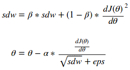
注意,这里的eps(epsilon)是为了数值稳定性而添加的,可以带入值10e-7。这会看上去如何呢?
import numpy as np

import matplotlib.mlab as mlab

import matplotlib.pyplot as plt

import scipy.stats

import matplotlib.animation as animation


def minimaFunction(params):

    #Bivariate Normal function

    X,Y = params


    sigma11,sigma12,mu11,mu12 = (3.0,.5,0.0,0.0)


    Z1 = mlab.bivariate_normal(X, Y, sigma11,sigma12,mu11,mu12)


    Z = Z1


    return -40*Z


def minimaFunctionDerivative(params):

    # Derivative of the bivariate normal function

    X,Y = params


    sigma11,sigma12,mu11,mu12 = (3.0,.5,0.0,0.0)


    dZ1X = -scipy.stats.norm.pdf(X, mu11, sigma11)*(mu11 - X)/sigma11**2

    dZ1Y = -scipy.stats.norm.pdf(Y, mu12, sigma12)*(mu12 - Y)/sigma12**2


    return (dZ1X,dZ1Y)


def optimize(iterations, oF, dOF,params,learningRate,beta):

    """

    computes the optimal value of params for a given objective function and its derivative

    Arguments:

        - iteratoins - the number of iterations required to optimize the objective function

        - oF - the objective function

        - dOF - the derivative function of the objective function

        - params - the parameters of the function to optimize

        - learningRate - the learning rate

- beta - The weighted moving average parameter for RMSProp

    Return:

        - oParams - the list of optimized parameters at each step of iteration

    """

    oParams = [params]

    sdw     = (0.0,0.0)

    eps = 10**(-7)

    #The iteration loop

    for i in range(iterations):

        # Compute the derivative of the parameters

        dParams = dOF(params)


        # Compute the momentum of each gradient sdw = sdw*beta+(1.0+beta)*dPar^2

        sdw = tuple([sDW*beta+(1.0-beta)*dPar**2 for dPar,sDW in zip(dParams,sdw)])


        #SGD in this line Goes through each parameter and applies parameter = parameter -learningrate*dParameter

        params = tuple([par-learningRate*dPar/((sDW**.5)+eps) for sDW,par,dPar in zip(sdw,params,dParams)])


        # append the new parameters

        oParams.append(params)


    return oParams


iterations=10

learningRate = .3

beta = .9

x,y = 5.0,1.0

params = (x,y)

optimizedParameters = optimize(iterations,\

                               minimaFunction,\

                               minimaFunctionDerivative,\

                               params,\

                               learningRate,\

                               beta)
Adam算法
Adam算法将Momentum算法和RMSProp算法的概念结合到一种算法中,以获得两种算法的最佳特征。它的公式如下: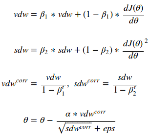
import numpy as np

import matplotlib.mlab as mlab

import matplotlib.pyplot as plt

import scipy.stats

import matplotlib.animation as animation


def minimaFunction(params):

    #Bivariate Normal function

    X,Y = params


    sigma11,sigma12,mu11,mu12 = (3.0,.5,0.0,0.0)


    Z1 = mlab.bivariate_normal(X, Y, sigma11,sigma12,mu11,mu12)


    Z = Z1


    return -40*Z


def minimaFunctionDerivative(params):

    # Derivative of the bivariate normal function

    X,Y = params


    sigma11,sigma12,mu11,mu12 = (3.0,.5,0.0,0.0)


    dZ1X = -scipy.stats.norm.pdf(X, mu11, sigma11)*(mu11 - X)/sigma11**2

    dZ1Y = -scipy.stats.norm.pdf(Y, mu12, sigma12)*(mu12 - Y)/sigma12**2


    return (dZ1X,dZ1Y)


def optimize(iterations, oF, dOF,params,learningRate,beta1,beta2):

    """

    computes the optimal value of params for a given objective function and its derivative

    Arguments:

        - iteratoins - the number of iterations required to optimize the objective function

        - oF - the objective function

        - dOF - the derivative function of the objective function

        - params - the parameters of the function to optimize

        - learningRate - the learning rate

- beta1 - The weighted moving average parameter for momentum component of ADAM

- beta2 - The weighted moving average parameter for RMSProp component of ADAM

    Return:

        - oParams - the list of optimized parameters at each step of iteration

    """

    oParams = [params]

    vdw     = (0.0,0.0)

    sdw     = (0.0,0.0)

    vdwCorr = (0.0,0.0)

    sdwCorr = (0.0,0.0)


    eps = 10**(-7)

    #The iteration loop

    for i in range(iterations):

        # Compute the derivative of the parameters

        dParams = dOF(params)


        # Compute the momentum of each gradient vdw = vdw*beta+(1.0+beta)*dPar

        vdw     = tuple([vDW*beta1+(1.0-beta1)*dPar for dPar,vDW in zip(dParams,vdw)])


        # Compute the rms of each gradient sdw = sdw*beta+(1.0+beta)*dPar^2

        sdw     = tuple([sDW*beta2+(1.0-beta2)*dPar**2.0 for dPar,sDW in zip(dParams,sdw)])

        # Compute the weight boosting for sdw and vdw

        vdwCorr = tuple([vDW/(1.0-beta1**(i+1.0)) for vDW in vdw])

        sdwCorr = tuple([sDW/(1.0-beta2**(i+1.0)) for sDW in sdw])


        #SGD in this line Goes through each parameter and applies parameter = parameter -learningrate*dParameter

        params = tuple([par-learningRate*vdwCORR/((sdwCORR**.5)+eps) for sdwCORR,vdwCORR,par in zip(vdwCorr,sdwCorr,params)])


        # append the new parameters

        oParams.append(params)


    return oParams


iterations=100

learningRate = .1

beta1 = .9

beta2 = .999

x,y = 5.0,1.0

params = (x,y)

optimizedParameters = optimize(iterations,\

                               minimaFunction,\

                               minimaFunctionDerivative,\

                               params,\

                               learningRate,\

                               beta1,\

                               beta2)
Adam算法可能是目前深度学习中最广泛使用的优化算法。它在各种各样的应用程序中都很好用。你会注意到,Adam算法计算的是一个vdwcorr值。这个值被用来“热身”指数的加权移动平均。通过推进这些值与经过的迭代次数成反比,它将标准化这些值。在使用Adam算法时,有一些很好的初始值。最好从一开始就将β1(beta1)设置为.9,β2(beta2)设置为.999。
结尾
在选择如何优化你的输入参数作为目标函数的一个函数时,你有相当多的选择。在上面的例子中,我们发现每种算法的收敛速度变得越来越快:
- 随机梯度下降算法:100次迭代
- 随机梯度下降算法+Momentum算法:50次迭代
- RMSProp算法:10次迭代
—Adam算法:5次迭代
代码地址:https://github.com/ManuelGonzalezRivero/3dbabove

欢迎关注ATYUN官方公众号
商务合作及内容投稿请联系邮箱:bd@atyun.com


广告


广告