


请先登录您的atyun账户,方可使用该功能

审核通过后即可使用此功能,请耐心等待~


深度学习视角下的扩散模型工作方式
2023年07月21日 由 Alex 发表
478727
0
本文是关于深度学习“扩散模型如何工作”的介绍。
简而言之,扩散模型是基于物理学的(想象一下,一杯水中有一滴墨水,起初你可以看到墨水滴落在哪里,但随着时间的推移,你会看到它在水中扩散,直到消失)。在本文中,我们需要创造8位精灵(游戏邦注:就像在Game Boy电子游戏《Pokemon Green Leaf》中所使用的精灵一样),如下所示:

当然,训练数据是精灵的图像,目标是生成更多的新精灵,扩散模型的工作方式是在图像中添加“噪声”,即所谓的“噪声处理”。
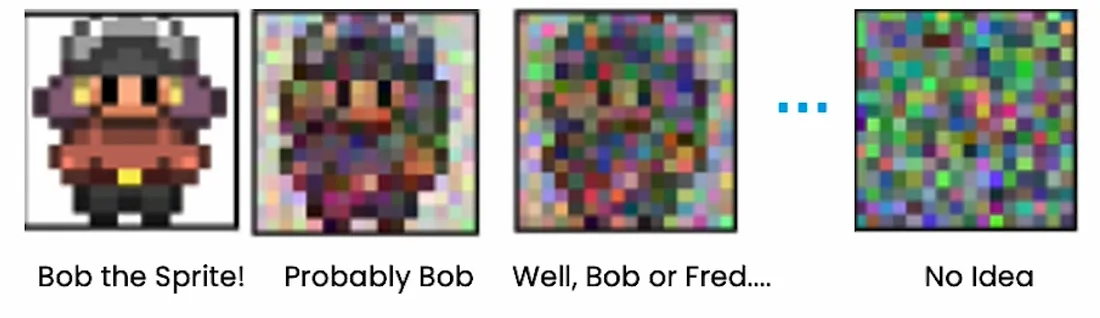
神经网络在这个示例中“思考”如下:
1. 如果是Bob精灵->让Bob保持原样
2. 如果可能是Bob->建议可能需要填写的细节
3. 如果是“好吧,Bob或Fred”->建议类似精灵的一般细节
4. 如果其总噪声->建议精灵的轮廓
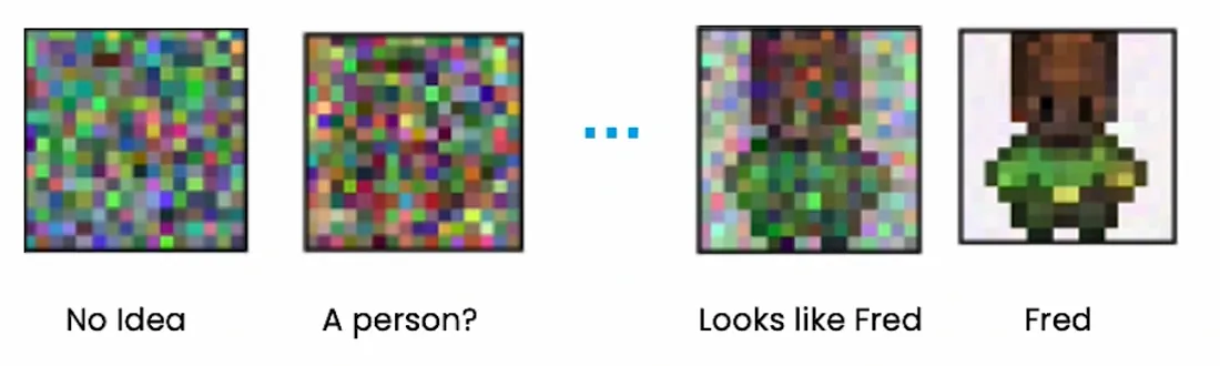
神经网络的训练部分是获取噪声图像并将其转化为精灵。学会消除你添加的噪音。
当你有一个完全噪声的图像时,噪声是正态分布的。
所以如果你想要一个新的精灵:
1. 正态分布的样本噪声
2. 使用网络去掉噪音得到一个全新的精灵
我们知道的是,神经网络试图预测每一步的噪声。神经网络知道精灵是什么样子,但预测的是噪声,而不是精灵本身,然后我们从原始噪声样本(正态分布)中减去预测的噪声,从而在每个时间步得到更接近精灵的东西。
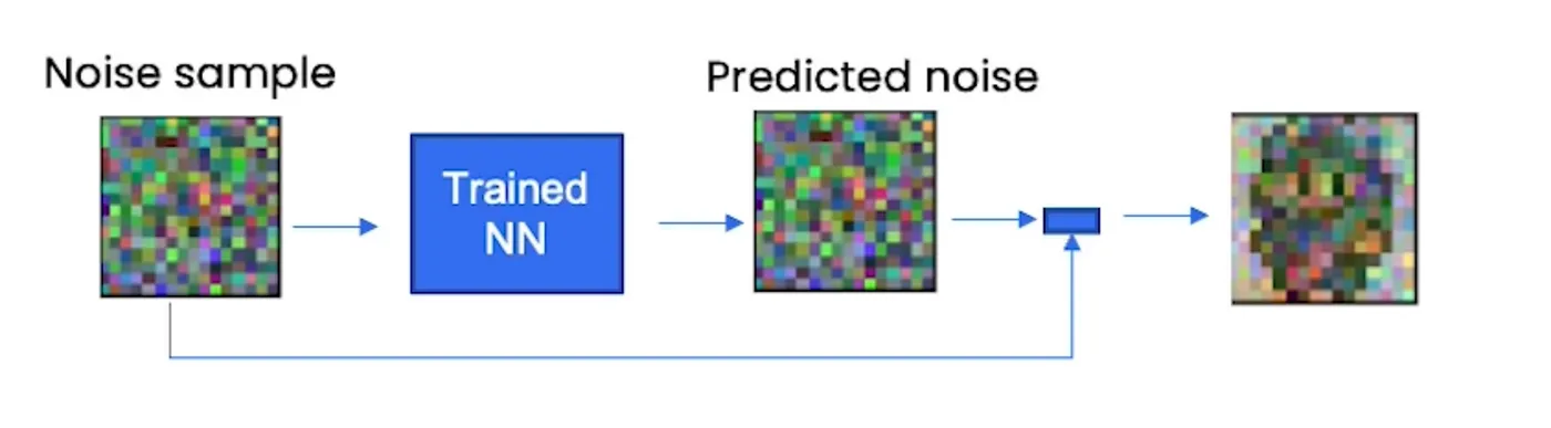
你需要多个步骤才能获得类似精灵的内容。
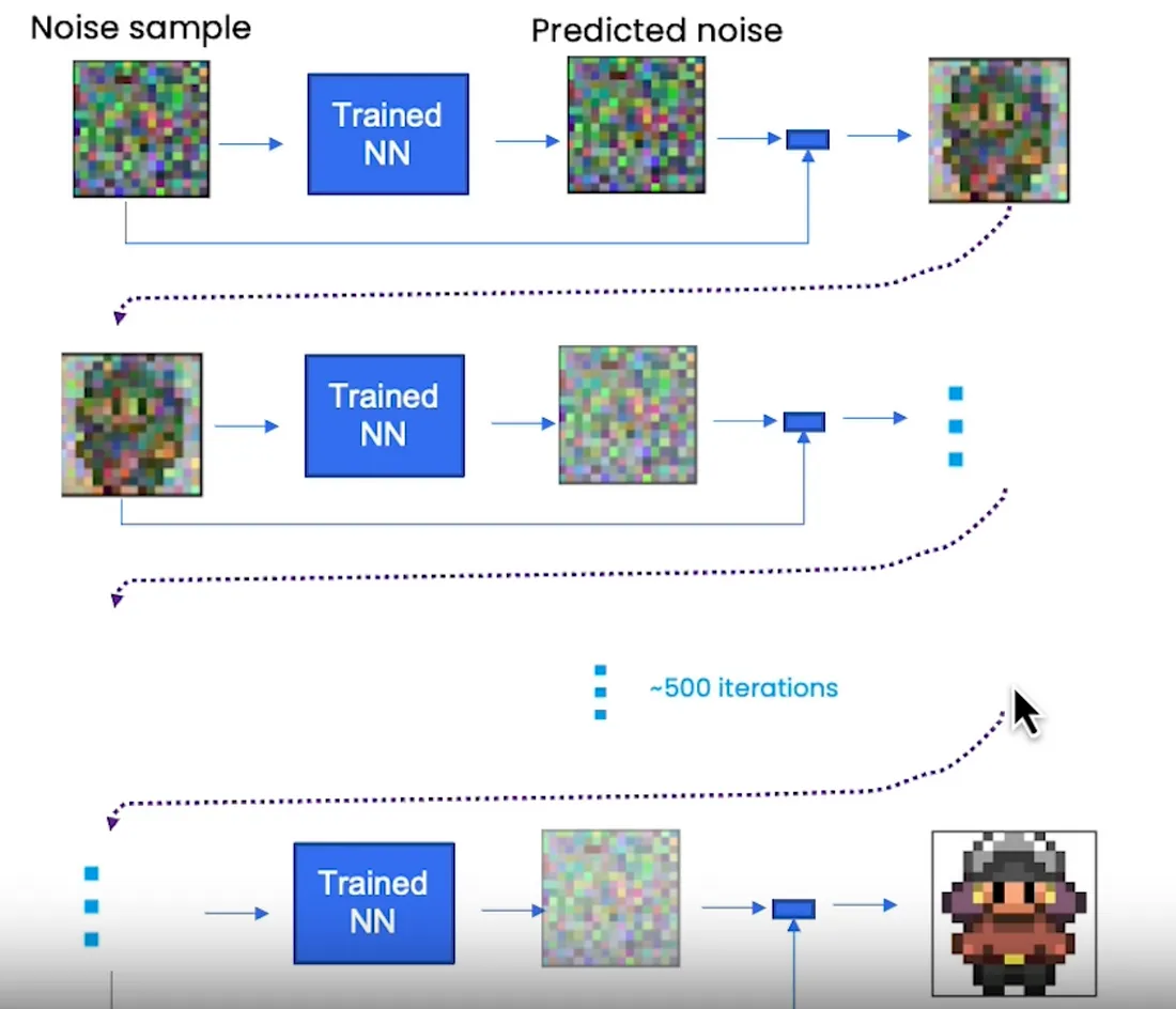
算法上看起来是这样的(伪代码):
在像这样的Python代码中,我们将攻击采样代码的每一行,但这只是一个预览:
所以我们使用PyTorch,让我们深入了解DDPM(去噪扩散概率模型)算法的每个部分。
将给出正态分布中噪声的初始样本;
torch.randn()函数用于从正态分布生成随机数张量。Randn (n_sample, 3, height, height).to(device)让我们一步步分解这个表达式:
1. torch.randn(…):创建一个张量,其中填充了从标准正态分布(平均值为0,标准差为1)中抽取的随机数。
2. (n_sample, 3, height, height):这个指定了张量的形状。它创建一个4维张量,其中包含了n_sample个样本,3个通道,以及高度为height的维度。
3. .to(device):如果可用,将张量移动到特定的设备(例如GPU)。device变量表示张量应该驻留的设备。如果一个GPU是可用的(torch.cuda.is_available()为True),它将被移动到GPU;否则,它将停留在CPU上。
把它们放在一起,torch.randn (n_sample, 3, height, height).to(device)生成具有指定形状的随机张量,并将其移动到所需的设备。
例如,如果n_sample = 10, height = 16,并且设备设置为使用GPU,则该表达式将生成一个形状为(10,3,16,16)的张量,其中填充了随机数,并将其移动到GPU。
然后你想穿越时间,从timesteps回到0,想想墨水滴的例子,我们想从完全扩散到开始。
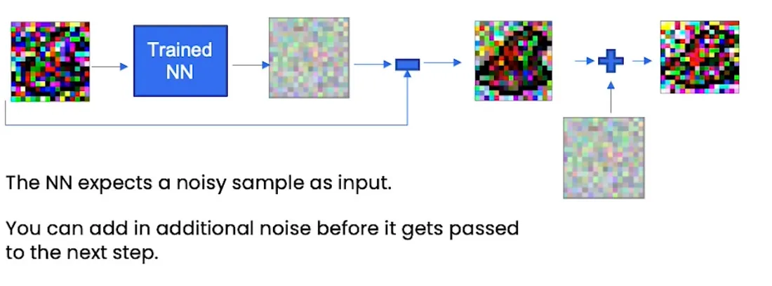
然后采样一些额外的噪声,我们稍后会回到“添加更多噪声”的部分。
然后用训练好的神经网络预测每个timesteps的噪声。记住这个噪声是神经网络想要从原始样本噪声中减去的噪声。
最后,DDPM算法就是从原始数据中减去pred_noise然后再加一点噪声。
现在,采样算法总体上我们可以继续构建神经网络并训练它。
我们将在实践中逐行解释这个算法。
假设你已经有了一个经过训练的神经网络。
代码如下:
让我们从头开始:
这是DDPM超参数,像任何其他ML/DL模型一样,beta1和beta2的正确值是没有正确答案的。
扩散模型中beta1和beta2的值可以通过实验和微调来确定。这些值控制在采样过程中每个timesteps加的噪声的大小。
通常,beta1是一个接近于零的小正值,如1e-4,而beta2是一个较大的值,介于0.01和0.1之间。beta1和beta2的具体值可以取决于数据集的特征和生成样本中所需的噪声水平。
为beta1和beta2寻找合适值的一种常用方法是执行网格搜索或试错实验。从beta1和beta2的值范围开始,并使用扩散模型生成样本。根据视觉吸引力、多样性或与训练数据的相似性等标准评估生成样本的质量。根据观察结果反复调整beta1和beta2的值,直到获得满意的样本。
PyTorch的说法:“如果有其他设备使用CPU,寻找cuda GPU”。
在扩散模型的上下文中,术语“n_feat”指的是神经网络模型中隐藏特征或隐藏维度的数量。
神经网络由多层组成,每层包含一定数量的隐藏单元或节点。这些隐藏单元负责捕获和表示输入数据中的复杂模式和特征。
参数“n_feat”指定扩散模型中使用的神经网络的特定层中隐藏特征或隐藏维度的数量。它决定了模型学习和表示数据中底层模式和结构的能力或复杂性。
“n_feat”的值越高,表示隐藏的特征数量越多,允许模型捕获数据中更复杂和细粒度的细节。然而,大量的隐藏特征也增加了模型的计算复杂度和内存需求。
“n_feat”值的选择取决于各种因素,包括数据的复杂性、可用的计算资源以及模型容量和效率之间所需的权衡。它通常是通过实验和微调来确定的,其中测试不同的“n_feat”值,以找到模型性能和计算效率之间的最佳平衡。
在扩散模型的上下文中,术语“n_cfeat”指的是上下文向量的大小或维度。上下文向量是神经网络模型的额外输入,它提供上下文信息或条件反射来影响生成过程。
上下文向量通常用于包含附加信息或指导基于特定属性或条件的样本生成。例如,在图像生成任务中,上下文向量可以对生成图像的所需类或样式等信息进行编码。
参数“n_cfeat”指定上下文向量的大小或维度。它确定上下文向量中用于约束生成过程的元素或特征的数量。
“n_cfeat”值的选择取决于具体的任务和需要合并的上下文信息的性质。它可以根据条件因素的复杂性和多样性而变化。例如,如果上下文向量表示二进制属性(例如,男性或女性),“n_cfeat”将被设置为2。如果上下文向量表示连续属性(例如,年龄),“n_cfeat”将被设置为捕获所需粒度级别的合适值。
上下文向量的大小影响模型捕获和利用上下文信息的能力。
该代码块为去噪扩散概率模型(DDPM)构建了噪声调度。它定义了三个张量:b_t, a_t和ab_t。噪声表决定了在每个扩散步骤中要添加的噪声级别。下面是每行的细分:
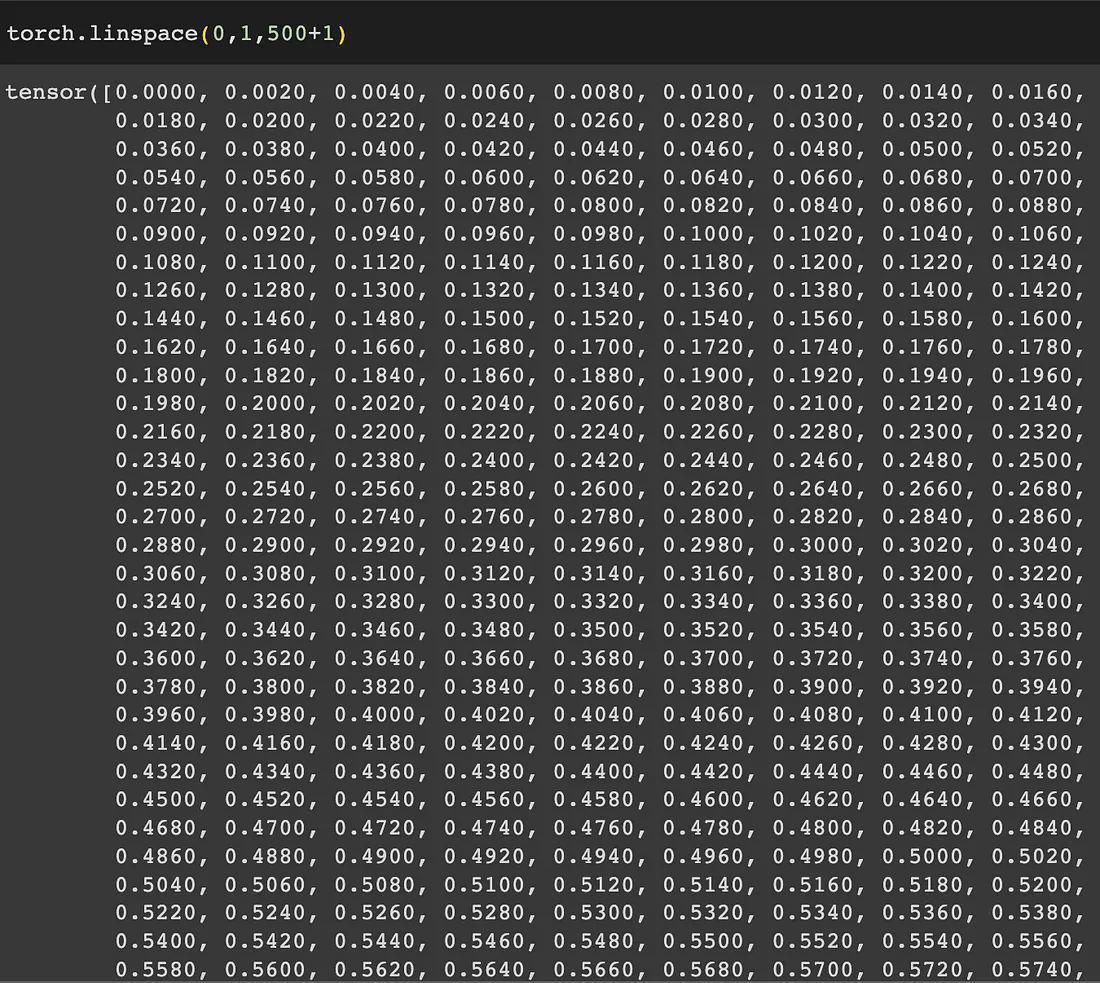
1. 第一行通过在0到1的范围内的timesteps + 1个间隔中对beta1和beta2进行线性插值来计算b_t。它使用torch.linspace创建了一系列等间距的值。
2. 第二行通过从1减去b_t来计算a_t。这保证了a_t和b_t的和总是1。
3. 第三行通过沿指定维度(可能是扩散步骤)对a_t的对数进行累积求和,然后对结果进行指数运算,计算出ab_t。这个累积和用于计算考虑到扩散过程每一步积累效应的因子。
4. 第四行将ab_t的第一个元素设置为1,确保初始因子为1。
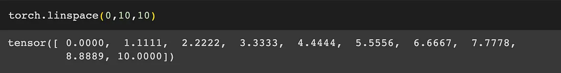
torch.linspace (range_start, range_end, interval)以n个间隔创建从range_start到range_end的等距值。然后乘以2减去1最后加上1。
显然:
Torch.cumsum()只是0轴(行)或1轴(列)的累积和。例:
我们做ab_t在0维上的对数值的累加和然后对每个值做指数计算。
让我们进一步分析:
1. a_t.log():计算张量a_t的逐元素对数(自然对数)。
2. torch.cumsum(a_t.log(), dim=0):这将沿着dim=0指定的维度对张量应用累积求和操作。它沿着第一个维度累积这些值,产生与输入张量形状相同的张量。
3. .exp():在计算累计和之后,使用.exp()函数按元素计算值求幂。此操作与前面执行的对数操作相反,有效地将值从对数尺度转换为原始尺度。
但是 Napo,如果稍后我们要使用 .exp() 来“反转”日志,为什么我们要在每个元素上执行 .log() 呢?
让我们再一步一步来分析:
1. a_t.log()计算张量a_t中每个元素的自然对数。对数函数记为log()。此操作是按元素执行的,这意味着要为张量中的每个单独的值计算对数。
2. 取对数的目的通常是将乘法运算转化为加法运算。在这种情况下,我们可以将a_t视为表示概率或权重,取对数将概率的乘法转换为对数概率的加法。这可以简化某些计算和数值稳定性。
3. .exp()应用于a_t.log()的结果。指数函数表示为exp(),是对数函数的倒数。应用指数函数有效地撤消了对数运算并恢复了原始值。
4. 在a_t.log()之后使用.exp()的目的是反转对数的效果并获得原始值。它把对数概率转换回概率。这一步是必要的,因为后续的计算或对ab_t的解释需要原始值,而不是对数转换后的值。
在给定的代码中,取对数(log())并应用指数函数(exp())用于与数值稳定性和计算效率相关的特定目的。它允许更稳定的计算,并防止在处理非常小或非常大的值时可能发生的数值下溢或溢出。
通过对这些值取对数,我们将它们从乘法尺度度转换为加法尺度。这可以通过多种方式帮助:
1. 稳定性:与原始尺度相比,对数可以处理更大范围的值。在对数域中工作有助于防止在计算过程中可能发生的数值下溢(非常小的值)或溢出(非常大的值)。
2. 计算效率:一些计算或模型,如神经网络中的梯度计算,在对数尺度上执行时效率更高。对数允许更简单的算术运算,比如加法,而不是乘法。
然而,当涉及到解释或使用结果时,我们通常需要将值转换回原始尺度,这就是为什么我们在取对数后应用指数函数(exp())。这一步允许我们恢复原始值并在原始上下文中使用它们。
综上所述,从原始尺度到对数尺度的转换是出于计算和数值稳定性的考虑。
这部分很短,因为我们只关注采样部分,但我们仍然可以看到使用的神经网络超参数。
此代码片段是扩散模型中使用的辅助函数。它的目的是从输入中去除预测的噪声,同时添加一些新的噪声,以避免信息崩溃或丢失。
这一行定义了一个名为denoise_add_noise的函数。它有四个参数:x,代表输入;T,表示当前扩散步长;Pred_noise,这是当前步骤的预测噪声;还有一个可选参数z,表示随机噪声。
这一行检查是否没有提供z。如果z未给定,则使用torch.randn_like(x)生成随机噪声,其中torch.randn_like()使用从标准正态分布中采样的随机值创建与x形状相同的张量,也就是像原始噪声一样的另一个样本。
这一行通过将b_t[t](我们之前声明的)的平方根乘以z来计算噪声。
这一行通过减去pred_noise乘以x中的某个表达式来计算平均值。该表达式涉及a_t和ab_t。
总之,代码基于参数beta1和beta2构造了一个噪声调度。然后,辅助函数denoise_add_noise使用这个噪声调度通过减去预测的噪声,同时根据噪声调度添加一些新的噪声来对输入x进行降噪。
我们只需加载预训练的模型权重并设置.eval()
在PyTorch中,nn_model.eval()方法用于将模型设置为求值模式。当将模型设置为评估模式时,它会影响模型中某些层或模块的行为,例如Dropout和批处理规范化。
在训练期间,模型通常包括Dropout和批处理规范化等层,它们在训练和评估期间的行为不同。Dropout随机地将一小部分输入单元设置为零,而批处理规范化通过使用批统计对输入进行规范化。
当你调用nn_model.eval()时,它将模型切换到求值模式,并相应地调整这些层/模块。具体地说:
1. 退出(Dropout):在评估过程中,退出层被关闭,所有单位被保留。这是因为我们想要使用整个网络来评估模型的性能,而不存在随机丢失。
2. 批量归一化:在评估过程中,批量归一化层使用训练期间计算的运行统计量(均值和方差)对输入进行归一化。这确保了培训和评估之间的一致行为。
通过使用nn_model.eval()将模型设置为评估模式,可以确保模型在推理或评估阶段的行为适当,从而提供与训练期间一致的结果。
值得注意的是,当你想恢复训练时,应该调用nn_model.train()将模型切换回训练模式。
在PyTorch中,@torch.no_grad()装饰器用于指定禁用梯度计算的上下文。它通常在执行推理或评估模型时使用,在这些情况下,我们不需要计算参数更新的梯度。
当一个代码块被@torch.no_grad()包装时,在该代码块内执行的任何操作都不会跟踪梯度计算的操作。这在计算效率方面是有益的,因为它避免了为反向传播存储中间值。
在提供的代码片段中,@torch.no_grad()被用作sample_ddpm函数的装饰器。说明在使用扩散模型生成样本时,不应计算或更新模型参数的梯度。因为生成样本不需要梯度信息,所以使用@torch.no_grad()可以帮助提高函数的性能和内存使用。
这只是为了重塑变量t或者“步长”;
创建一个张量t,表示扩散模型中的当前timesteps。让我们进一步分析:
1. i表示for循环中的当前迭代,它从timesteps迭代到1。
2. timesteps是扩散模型中timesteps的总数。
为了计算t的值,我们将i除以timesteps,使其在0到1之间归一化。这种归一化是为了确保t在整个扩散过程中保持在有效范围内。
代码[i / timesteps]创建一个包含规范化timesteps值的列表。方括号[]在Python中表示一个列表。
下一部分[:,None, None, None]用于将列表重塑为张量。让我们一步一步来理解:
1. [:, None]向张量添加一个额外的维度。冒号:表示我们希望将所有元素保留在第一个维度中(在本例中只有一个元素),None在该位置添加一个新维度。这种重塑允许张量具有(1,1)的形状。
2. 该过程再重复两次,使用None来进一步扩展维度,得到一个张量形状(1,1,1,1)。
最后,.to(device)用于在可用的情况下将张量移动到指定的设备(例如GPU)。这确保张量在选定的设备上被存储和处理。
时间例子:
1. 迭代:假设我们在循环的中间,并且i=250。
2. 归一化:我们用i(250)除以timesteps(500)来归一化0到1之间的值。结果是0.5。
3. 张量创建:代码[i ,timesteps]创建一个具有标准化timesteps值[0.5]的列表。
4. 重塑:接下来,我们应用[:,None, None, None]将列表重塑为张量。发生情况如下:
5. 设备传输:最后,.to(Device)用于将张量移动到指定的设备,如GPU,如果可用的话。这确保张量在选定的设备上被存储和处理。
创建标记后添加的extra_noise
该模型试图预测每个timesteps的噪声
通过刚才的函数,我们从原始噪声中移除noise_pred,然后再添加一点。
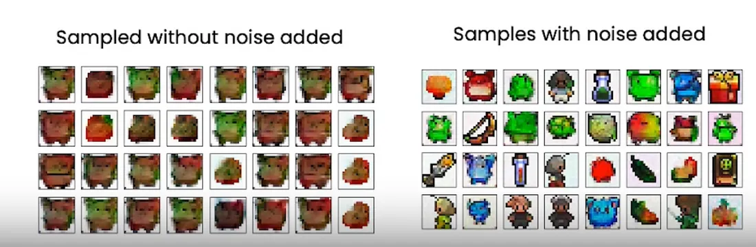
如果你不能 100% 确定为什么我们添加一点比例噪声,是因为我们避免预测只是数据集的平均值并为我们提供“blob”精灵。为什么?
因为NN期望噪声来自正态分布,当我们从OG噪声中减去NN的noise_pred后,我们就不再是正态分布的噪声了,所以我们添加了噪声。
用于扩散模型的神经网络现在也用于图像分割,即所谓的U-Net,但经过调整后添加了上下文,因此在这种情况下它实际上被称为“ContextU-Net”。理解这个神经网络很重要的一点是它的输出和输入是一样的。所以在这种情况下,输入是一个16×16像素的精灵图像,输出是一个16×16图像(或表示该16×16图像的张量)中的预测噪声。
来源:https://medium.com/@sergio.leal/how-diffusion-models-work-by-deeplearning-ai-recap-c66de2e19d71
直觉
简而言之,扩散模型是基于物理学的(想象一下,一杯水中有一滴墨水,起初你可以看到墨水滴落在哪里,但随着时间的推移,你会看到它在水中扩散,直到消失)。在本文中,我们需要创造8位精灵(游戏邦注:就像在Game Boy电子游戏《Pokemon Green Leaf》中所使用的精灵一样),如下所示:
当然,训练数据是精灵的图像,目标是生成更多的新精灵,扩散模型的工作方式是在图像中添加“噪声”,即所谓的“噪声处理”。
神经网络在这个示例中“思考”如下:
1. 如果是Bob精灵->让Bob保持原样
2. 如果可能是Bob->建议可能需要填写的细节
3. 如果是“好吧,Bob或Fred”->建议类似精灵的一般细节
4. 如果其总噪声->建议精灵的轮廓
神经网络的训练部分是获取噪声图像并将其转化为精灵。学会消除你添加的噪音。
当你有一个完全噪声的图像时,噪声是正态分布的。
所以如果你想要一个新的精灵:
1. 正态分布的样本噪声
2. 使用网络去掉噪音得到一个全新的精灵
采样
我们知道的是,神经网络试图预测每一步的噪声。神经网络知道精灵是什么样子,但预测的是噪声,而不是精灵本身,然后我们从原始噪声样本(正态分布)中减去预测的噪声,从而在每个时间步得到更接近精灵的东西。
你需要多个步骤才能获得类似精灵的内容。
算法上看起来是这样的(伪代码):
sample = random_sample

for t=T,...,1 do:

    extra_noise = random_sample if t > 1 else extra_noise = 0

    predicted_noise = trained_nn(x_t-1,t)

    s1,s2,s3 = ddpm_scaling(t)

    sample = s1 * (sample - s2 * predicted_noise) + s3 * extra_noise
在像这样的Python代码中,我们将攻击采样代码的每一行,但这只是一个预览:
# sample using standard algorithm

@torch.no_grad()

def sample_ddpm(n_sample, save_rate=20):

    # x_T ~ N(0, 1), sample initial noise

    samples = torch.randn(n_sample, 3, height, height).to(device)


    for i in range(timesteps, 0, -1):

        print(f'sampling timestep {i:3d}', end='\r')


        # reshape time tensor

        t = torch.tensor([i / timesteps])[:, None, None, None].to(device)


        # sample some random noise to inject back in. For i = 1, don't add back in noise

        z = torch.randn_like(samples) if i > 1 else 0


        eps = nn_model(samples, t) # predict noise e_(x_t,t)

        samples = denoise_add_noise(samples, i, eps, z)


    return samples
所以我们使用PyTorch,让我们深入了解DDPM(去噪扩散概率模型)算法的每个部分。
samples = torch.randn(n_sample, 3, height, height).to(device)
将给出正态分布中噪声的初始样本;
torch.randn()函数用于从正态分布生成随机数张量。Randn (n_sample, 3, height, height).to(device)让我们一步步分解这个表达式:
1. torch.randn(…):创建一个张量,其中填充了从标准正态分布(平均值为0,标准差为1)中抽取的随机数。
2. (n_sample, 3, height, height):这个指定了张量的形状。它创建一个4维张量,其中包含了n_sample个样本,3个通道,以及高度为height的维度。
3. .to(device):如果可用,将张量移动到特定的设备(例如GPU)。device变量表示张量应该驻留的设备。如果一个GPU是可用的(torch.cuda.is_available()为True),它将被移动到GPU;否则,它将停留在CPU上。
把它们放在一起,torch.randn (n_sample, 3, height, height).to(device)生成具有指定形状的随机张量,并将其移动到所需的设备。
例如,如果n_sample = 10, height = 16,并且设备设置为使用GPU,则该表达式将生成一个形状为(10,3,16,16)的张量,其中填充了随机数,并将其移动到GPU。
for i in range(timesteps, 0, -1):
然后你想穿越时间,从timesteps回到0,想想墨水滴的例子,我们想从完全扩散到开始。
z = torch.randn_like(samples) if i > 1 else 0
然后采样一些额外的噪声,我们稍后会回到“添加更多噪声”的部分。
eps = nn_model(samples, t)
然后用训练好的神经网络预测每个timesteps的噪声。记住这个噪声是神经网络想要从原始样本噪声中减去的噪声。
samples = denoise_add_noise(samples, i, eps, z)
最后,DDPM算法就是从原始数据中减去pred_noise然后再加一点噪声。
现在,采样算法总体上我们可以继续构建神经网络并训练它。
我们将在实践中逐行解释这个算法。
假设你已经有了一个经过训练的神经网络。
代码如下:
# hyperparameters


# diffusion hyperparameters

timesteps = 500

beta1 = 1e-4

beta2 = 0.02


# network hyperparameters

device = torch.device("cuda:0" if torch.cuda.is_available() else torch.device('cpu'))

n_feat = 64 # 64 hidden dimension feature

n_cfeat = 5 # context vector is of size 5

height = 16 # 16x16 image

save_dir = './weights/'


# construct DDPM noise schedule

b_t = (beta2 - beta1) * torch.linspace(0, 1, timesteps + 1, device=device) + beta1

a_t = 1 - b_t

ab_t = torch.cumsum(a_t.log(), dim=0).exp()

ab_t[0] = 1


# construct model

nn_model = ContextUnet(in_channels=3, n_feat=n_feat, n_cfeat=n_cfeat, height=height).to(device)


# helper function; removes the predicted noise (but adds some noise back in to avoid collapse)

def denoise_add_noise(x, t, pred_noise, z=None):

    if z is None:

       z = torch.randn_like(x)

    noise = b_t.sqrt()[t] * z

    mean = (x - pred_noise * ((1 - a_t[t]) / (1 - ab_t[t]).sqrt())) / a_t[t].sqrt()

    return mean + noise


# load in model weights and set to eval mode

nn_model.load_state_dict(torch.load(f"{save_dir}/model_trained.pth", map_location=device))

nn_model.eval()


# sample using standard algorithm

@torch.no_grad()

def sample_ddpm(n_sample, save_rate=20):

    # x_T ~ N(0, 1), sample initial noise

    samples = torch.randn(n_sample, 3, height, height).to(device)


    # array to keep track of generated steps for plotting

    intermediate = []

    for i in range(timesteps, 0, -1):

        print(f'sampling timestep {i:3d}', end='\r')


        # reshape time tensor

        t = torch.tensor([i / timesteps])[:, None, None, None].to(device)


        # sample some random noise to inject back in. For i = 1, don't add back in noise

        z = torch.randn_like(samples) if i > 1 else 0


        eps = nn_model(samples, t) # predict noise e_(x_t,t)

        samples = denoise_add_noise(samples, i, eps, z)

        if i % save_rate ==0 or i==timesteps or i<8:

           intermediate.append(samples.detach().cpu().numpy())


    intermediate = np.stack(intermediate)

    return samples, intermediate
第1部分:超参数变量
让我们从头开始:
# diffusion hyperparameters

timesteps = 500

beta1 = 1e-4

beta2 = 0.02
这是DDPM超参数,像任何其他ML/DL模型一样,beta1和beta2的正确值是没有正确答案的。
扩散模型中beta1和beta2的值可以通过实验和微调来确定。这些值控制在采样过程中每个timesteps加的噪声的大小。
通常,beta1是一个接近于零的小正值,如1e-4,而beta2是一个较大的值,介于0.01和0.1之间。beta1和beta2的具体值可以取决于数据集的特征和生成样本中所需的噪声水平。
为beta1和beta2寻找合适值的一种常用方法是执行网格搜索或试错实验。从beta1和beta2的值范围开始,并使用扩散模型生成样本。根据视觉吸引力、多样性或与训练数据的相似性等标准评估生成样本的质量。根据观察结果反复调整beta1和beta2的值,直到获得满意的样本。
第2部分:神经网络超参数
# network hyperparameters

device = torch.device("cuda:0" if torch.cuda.is_available() else torch.device('cpu'))

n_feat = 64 # 64 hidden dimension feature

n_cfeat = 5 # context vector is of size 5

height = 16 # 16x16 image

save_dir = './weights/'
device = torch.device("cuda:0" if torch.cuda.is_available() else torch.device('cpu'))PyTorch的说法:“如果有其他设备使用CPU,寻找cuda GPU”。
n_feat = 64 # 64 hidden dimension feature
在扩散模型的上下文中,术语“n_feat”指的是神经网络模型中隐藏特征或隐藏维度的数量。
神经网络由多层组成,每层包含一定数量的隐藏单元或节点。这些隐藏单元负责捕获和表示输入数据中的复杂模式和特征。
参数“n_feat”指定扩散模型中使用的神经网络的特定层中隐藏特征或隐藏维度的数量。它决定了模型学习和表示数据中底层模式和结构的能力或复杂性。
“n_feat”的值越高,表示隐藏的特征数量越多,允许模型捕获数据中更复杂和细粒度的细节。然而,大量的隐藏特征也增加了模型的计算复杂度和内存需求。
“n_feat”值的选择取决于各种因素,包括数据的复杂性、可用的计算资源以及模型容量和效率之间所需的权衡。它通常是通过实验和微调来确定的,其中测试不同的“n_feat”值,以找到模型性能和计算效率之间的最佳平衡。
n_cfeat = 5 # context vector is of size 5
在扩散模型的上下文中,术语“n_cfeat”指的是上下文向量的大小或维度。上下文向量是神经网络模型的额外输入,它提供上下文信息或条件反射来影响生成过程。
上下文向量通常用于包含附加信息或指导基于特定属性或条件的样本生成。例如,在图像生成任务中,上下文向量可以对生成图像的所需类或样式等信息进行编码。
参数“n_cfeat”指定上下文向量的大小或维度。它确定上下文向量中用于约束生成过程的元素或特征的数量。
“n_cfeat”值的选择取决于具体的任务和需要合并的上下文信息的性质。它可以根据条件因素的复杂性和多样性而变化。例如,如果上下文向量表示二进制属性(例如,男性或女性),“n_cfeat”将被设置为2。如果上下文向量表示连续属性(例如,年龄),“n_cfeat”将被设置为捕获所需粒度级别的合适值。
上下文向量的大小影响模型捕获和利用上下文信息的能力。
第3部:DDPM噪声表
# construct DDPM noise schedule

b_t = (beta2 - beta1) * torch.linspace(0, 1, timesteps + 1, device=device) + beta1

a_t = 1 - b_t

ab_t = torch.cumsum(a_t.log(), dim=0).exp()

ab_t[0] = 1
该代码块为去噪扩散概率模型(DDPM)构建了噪声调度。它定义了三个张量:b_t, a_t和ab_t。噪声表决定了在每个扩散步骤中要添加的噪声级别。下面是每行的细分:
1. 第一行通过在0到1的范围内的timesteps + 1个间隔中对beta1和beta2进行线性插值来计算b_t。它使用torch.linspace创建了一系列等间距的值。
2. 第二行通过从1减去b_t来计算a_t。这保证了a_t和b_t的和总是1。
3. 第三行通过沿指定维度(可能是扩散步骤)对a_t的对数进行累积求和,然后对结果进行指数运算,计算出ab_t。这个累积和用于计算考虑到扩散过程每一步积累效应的因子。
4. 第四行将ab_t的第一个元素设置为1,确保初始因子为1。
b_t = (beta2 - beta1) * torch.linspace(0, 1, timesteps + 1, device=device) + beta1
torch.linspace (range_start, range_end, interval)以n个间隔创建从range_start到range_end的等距值。然后乘以2减去1最后加上1。
a_t = 1 - b_t
显然:
Ab_t = torch.cumsum(a_t.log(), dim=0).exp()


Ab_t [0] = 1
Torch.cumsum()只是0轴(行)或1轴(列)的累积和。例:
x = torch.tensor([[1, 2, 3, 4],

                 [5, 6, 7, 8],

                 [9, 10, 11, 12]])


torch.cumsum(x, dim=0) # This will print:


tensor([[ 1, 2, 3, 4],

       [ 6, 8, 10, 12],

       [15, 18, 21, 24]])


torch.cumsum(x, dim=1) # will print this:


tensor([[ 1, 3, 6, 10],

       [ 5, 11, 18, 26],

       [ 9, 19, 30, 42]])
我们做ab_t在0维上的对数值的累加和然后对每个值做指数计算。
让我们进一步分析:
1. a_t.log():计算张量a_t的逐元素对数(自然对数)。
2. torch.cumsum(a_t.log(), dim=0):这将沿着dim=0指定的维度对张量应用累积求和操作。它沿着第一个维度累积这些值,产生与输入张量形状相同的张量。
3. .exp():在计算累计和之后,使用.exp()函数按元素计算值求幂。此操作与前面执行的对数操作相反,有效地将值从对数尺度转换为原始尺度。
但是 Napo,如果稍后我们要使用 .exp() 来“反转”日志,为什么我们要在每个元素上执行 .log() 呢?
让我们再一步一步来分析:
1. a_t.log()计算张量a_t中每个元素的自然对数。对数函数记为log()。此操作是按元素执行的,这意味着要为张量中的每个单独的值计算对数。
2. 取对数的目的通常是将乘法运算转化为加法运算。在这种情况下,我们可以将a_t视为表示概率或权重,取对数将概率的乘法转换为对数概率的加法。这可以简化某些计算和数值稳定性。
3. .exp()应用于a_t.log()的结果。指数函数表示为exp(),是对数函数的倒数。应用指数函数有效地撤消了对数运算并恢复了原始值。
4. 在a_t.log()之后使用.exp()的目的是反转对数的效果并获得原始值。它把对数概率转换回概率。这一步是必要的,因为后续的计算或对ab_t的解释需要原始值,而不是对数转换后的值。
在给定的代码中,取对数(log())并应用指数函数(exp())用于与数值稳定性和计算效率相关的特定目的。它允许更稳定的计算,并防止在处理非常小或非常大的值时可能发生的数值下溢或溢出。
通过对这些值取对数,我们将它们从乘法尺度度转换为加法尺度。这可以通过多种方式帮助:
1. 稳定性:与原始尺度相比,对数可以处理更大范围的值。在对数域中工作有助于防止在计算过程中可能发生的数值下溢(非常小的值)或溢出(非常大的值)。
2. 计算效率:一些计算或模型,如神经网络中的梯度计算,在对数尺度上执行时效率更高。对数允许更简单的算术运算,比如加法,而不是乘法。
然而,当涉及到解释或使用结果时,我们通常需要将值转换回原始尺度,这就是为什么我们在取对数后应用指数函数(exp())。这一步允许我们恢复原始值并在原始上下文中使用它们。
综上所述,从原始尺度到对数尺度的转换是出于计算和数值稳定性的考虑。
第4部分:模型
这部分很短,因为我们只关注采样部分,但我们仍然可以看到使用的神经网络超参数。
# construct model

nn_model = ContextUnet(in_channels=3, n_feat=n_feat, n_cfeat=n_cfeat, height=height).to(device)
第5部分:去噪样本,然后再次添加噪声
def denoise_add_noise(x, t, pred_noise, z=None):

    if z is None:

    z = torch.randn_like(x)

    noise = b_t.sqrt()[t] * z

    mean = (x - pred_noise * ((1 - a_t[t]) / (1 - ab_t[t]).sqrt())) / a_t[t].sqrt()

    return mean + noise
此代码片段是扩散模型中使用的辅助函数。它的目的是从输入中去除预测的噪声,同时添加一些新的噪声,以避免信息崩溃或丢失。
def denoise_add_noise(x, t, pred_noise, z=None):
这一行定义了一个名为denoise_add_noise的函数。它有四个参数:x,代表输入;T,表示当前扩散步长;Pred_noise,这是当前步骤的预测噪声;还有一个可选参数z,表示随机噪声。
if z is None:

   z = torch.randn_like(x)
这一行检查是否没有提供z。如果z未给定,则使用torch.randn_like(x)生成随机噪声,其中torch.randn_like()使用从标准正态分布中采样的随机值创建与x形状相同的张量,也就是像原始噪声一样的另一个样本。
noise = b_t.sqrt()[t] * z
这一行通过将b_t[t](我们之前声明的)的平方根乘以z来计算噪声。
mean = (x - pred_noise * ((1 - a_t[t]) / (1 - ab_t[t]).sqrt())) / a_t[t].sqrt()
这一行通过减去pred_noise乘以x中的某个表达式来计算平均值。该表达式涉及a_t和ab_t。
总之,代码基于参数beta1和beta2构造了一个噪声调度。然后,辅助函数denoise_add_noise使用这个噪声调度通过减去预测的噪声,同时根据噪声调度添加一些新的噪声来对输入x进行降噪。
第6部分:加载权重和eval_mode()
nn_model.load_state_dict(torch.load(f"{save_dir}/model_trained.pth", map_location=device))

nn_model.eval()
我们只需加载预训练的模型权重并设置.eval()
在PyTorch中,nn_model.eval()方法用于将模型设置为求值模式。当将模型设置为评估模式时,它会影响模型中某些层或模块的行为,例如Dropout和批处理规范化。
在训练期间,模型通常包括Dropout和批处理规范化等层,它们在训练和评估期间的行为不同。Dropout随机地将一小部分输入单元设置为零,而批处理规范化通过使用批统计对输入进行规范化。
当你调用nn_model.eval()时,它将模型切换到求值模式,并相应地调整这些层/模块。具体地说:
1. 退出(Dropout):在评估过程中,退出层被关闭,所有单位被保留。这是因为我们想要使用整个网络来评估模型的性能,而不存在随机丢失。
2. 批量归一化:在评估过程中,批量归一化层使用训练期间计算的运行统计量(均值和方差)对输入进行归一化。这确保了培训和评估之间的一致行为。
通过使用nn_model.eval()将模型设置为评估模式,可以确保模型在推理或评估阶段的行为适当,从而提供与训练期间一致的结果。
值得注意的是,当你想恢复训练时,应该调用nn_model.train()将模型切换回训练模式。
第7部分:实际进行抽样并将所有内容组合在一起
@torch.no_grad()

def sample_ddpm(n_sample):

    # x_T ~ N(0, 1), sample initial noise

    samples = torch.randn(n_sample, 3, height, height).to(device)


    for i in range(timesteps, 0, -1):

        print(f'sampling timestep {i:3d}', end='\r')


        # reshape time tensor

        t = torch.tensor([i / timesteps])[:, None, None, None].to(device)


        # sample some random noise to inject back in. For i = 1, don't add back in noise

        z = torch.randn_like(samples) if i > 1 else 0


        eps = nn_model(samples, t) # predict noise e_(x_t,t)

        samples = denoise_add_noise(samples, i, eps, z)


    return samples
在PyTorch中,@torch.no_grad()装饰器用于指定禁用梯度计算的上下文。它通常在执行推理或评估模型时使用,在这些情况下,我们不需要计算参数更新的梯度。
当一个代码块被@torch.no_grad()包装时,在该代码块内执行的任何操作都不会跟踪梯度计算的操作。这在计算效率方面是有益的,因为它避免了为反向传播存储中间值。
在提供的代码片段中,@torch.no_grad()被用作sample_ddpm函数的装饰器。说明在使用扩散模型生成样本时,不应计算或更新模型参数的梯度。因为生成样本不需要梯度信息,所以使用@torch.no_grad()可以帮助提高函数的性能和内存使用。
t = torch.tensor([i / timesteps])[:, None, None, None].to(device)
这只是为了重塑变量t或者“步长”;
创建一个张量t,表示扩散模型中的当前timesteps。让我们进一步分析:
1. i表示for循环中的当前迭代,它从timesteps迭代到1。
2. timesteps是扩散模型中timesteps的总数。
为了计算t的值,我们将i除以timesteps,使其在0到1之间归一化。这种归一化是为了确保t在整个扩散过程中保持在有效范围内。
代码[i / timesteps]创建一个包含规范化timesteps值的列表。方括号[]在Python中表示一个列表。
下一部分[:,None, None, None]用于将列表重塑为张量。让我们一步一步来理解:
1. [:, None]向张量添加一个额外的维度。冒号:表示我们希望将所有元素保留在第一个维度中(在本例中只有一个元素),None在该位置添加一个新维度。这种重塑允许张量具有(1,1)的形状。
2. 该过程再重复两次,使用None来进一步扩展维度,得到一个张量形状(1,1,1,1)。
最后,.to(device)用于在可用的情况下将张量移动到指定的设备(例如GPU)。这确保张量在选定的设备上被存储和处理。
时间例子:
1. 迭代:假设我们在循环的中间,并且i=250。
2. 归一化:我们用i(250)除以timesteps(500)来归一化0到1之间的值。结果是0.5。
3. 张量创建:代码[i ,timesteps]创建一个具有标准化timesteps值[0.5]的列表。
4. 重塑:接下来,我们应用[:,None, None, None]将列表重塑为张量。发生情况如下:
①. [:, None]添加了一个额外的维度,结果为[[0.5]]。
②. 再次应用[:,None],得到[[[0.5]]]。
③. 再应用一次[:,None],得到[[[[0.5]]]]。那么,张量t现在的形状是(1,1,1,1)
5. 设备传输:最后,.to(Device)用于将张量移动到指定的设备,如GPU,如果可用的话。这确保张量在选定的设备上被存储和处理。
z = torch.randn_like(samples) if i > 1 else 0
创建标记后添加的extra_noise
eps = nn_model(samples, t)
该模型试图预测每个timesteps的噪声
samples = denoise_add_noise(samples, i, eps, z)
通过刚才的函数,我们从原始噪声中移除noise_pred,然后再添加一点。
如果你不能 100% 确定为什么我们添加一点比例噪声,是因为我们避免预测只是数据集的平均值并为我们提供“blob”精灵。为什么?
因为NN期望噪声来自正态分布,当我们从OG噪声中减去NN的noise_pred后,我们就不再是正态分布的噪声了,所以我们添加了噪声。
神经网络
用于扩散模型的神经网络现在也用于图像分割,即所谓的U-Net,但经过调整后添加了上下文,因此在这种情况下它实际上被称为“ContextU-Net”。理解这个神经网络很重要的一点是它的输出和输入是一样的。所以在这种情况下,输入是一个16×16像素的精灵图像,输出是一个16×16图像(或表示该16×16图像的张量)中的预测噪声。
class ContextUnet(nn.Module):

    def __init__(self, in_channels, n_feat=256, n_cfeat=10, height=28): # cfeat - context features

        super(ContextUnet, self).__init__()


        # number of input channels, number of intermediate feature maps and number of classes

        self.in_channels = in_channels

        self.n_feat = n_feat

        self.n_cfeat = n_cfeat

        self.h = height #assume h == w. must be divisible by 4, so 28,24,20,16...


        # Initialize the initial convolutional layer

        self.init_conv = ResidualConvBlock(in_channels, n_feat, is_res=True)


        # Initialize the down-sampling path of the U-Net with two levels

        self.down1 = UnetDown(n_feat, n_feat) # down1 #[10, 256, 8, 8]

        self.down2 = UnetDown(n_feat, 2 * n_feat) # down2 #[10, 256, 4, 4]


        # original: self.to_vec = nn.Sequential(nn.AvgPool2d(7), nn.GELU())

        self.to_vec = nn.Sequential(nn.AvgPool2d((4)), nn.GELU())


        # Embed the timestep and context labels with a one-layer fully connected neural network

        self.timeembed1 = EmbedFC(1, 2*n_feat)

        self.timeembed2 = EmbedFC(1, 1*n_feat)

        self.contextembed1 = EmbedFC(n_cfeat, 2*n_feat)

        self.contextembed2 = EmbedFC(n_cfeat, 1*n_feat)


        # Initialize the up-sampling path of the U-Net with three levels

        self.up0 = nn.Sequential(

            nn.ConvTranspose2d(2 * n_feat, 2 * n_feat, self.h//4, self.h//4), # up-sample

            nn.GroupNorm(8, 2 * n_feat), # normalize

            nn.ReLU(),

        )

        self.up1 = UnetUp(4 * n_feat, n_feat)

        self.up2 = UnetUp(2 * n_feat, n_feat)


        # Initialize the final convolutional layers to map to the same number of channels as the input image

        self.out = nn.Sequential(

            nn.Conv2d(2 * n_feat, n_feat, 3, 1, 1), # reduce number of feature maps #in_channels, out_channels, kernel_size, stride=1, padding=0

            nn.GroupNorm(8, n_feat), # normalize

            nn.ReLU(),

            nn.Conv2d(n_feat, self.in_channels, 3, 1, 1), # map to same number of channels as input

        )


        def forward(self, x, t, c=None):

            """

            x : (batch, n_feat, h, w) : input image

            t : (batch, n_cfeat) : time step

            c : (batch, n_classes) : context label

            """

            # x is the input image, c is the context label, t is the timestep, context_mask says which samples to block the context on


            # pass the input image through the initial convolutional layer

            x = self.init_conv(x)

            # pass the result through the down-sampling path

            down1 = self.down1(x) #[10, 256, 8, 8]

            down2 = self.down2(down1) #[10, 256, 4, 4]


            # convert the feature maps to a vector and apply an activation

            hiddenvec = self.to_vec(down2)


            # mask out context if context_mask == 1

            if c is None:

               c = torch.zeros(x.shape[0], self.n_cfeat).to(x)


            # embed context and timestep

            cemb1 = self.contextembed1(c).view(-1, self.n_feat * 2, 1, 1) # (batch, 2*n_feat, 1,1)

            temb1 = self.timeembed1(t).view(-1, self.n_feat * 2, 1, 1)

            cemb2 = self.contextembed2(c).view(-1, self.n_feat, 1, 1)

            temb2 = self.timeembed2(t).view(-1, self.n_feat, 1, 1)

            #print(f"uunet forward: cemb1 {cemb1.shape}. temb1 {temb1.shape}, cemb2 {cemb2.shape}. temb2 {temb2.shape}")

            up1 = self.up0(hiddenvec)

            up2 = self.up1(cemb1*up1 + temb1, down2) # add and multiply embeddings

            up3 = self.up2(cemb2*up2 + temb2, down1)

            out = self.out(torch.cat((up3, x), 1))

            return out
来源:https://medium.com/@sergio.leal/how-diffusion-models-work-by-deeplearning-ai-recap-c66de2e19d71

欢迎关注ATYUN官方公众号
商务合作及内容投稿请联系邮箱:bd@atyun.com


广告


写评论取消
回复取消