


请先登录您的atyun账户,方可使用该功能

审核通过后即可使用此功能,请耐心等待~


在Python中使用LIME框架:建立对机器学习模型的信任
2017年07月19日 由 xiaoshan.xiang 发表
986497
0
价值不在于软件,价值在于数据,这对每一家公司而言都是非常重要的,他们了解他们拥有的数据。
现在越来越多的公司意识到数据的强大。机器学习模型越来越受欢迎,现在正在使用数据来解决各种商业问题。话虽如此,模型的准确性和可解释性之间总是存在着取舍。
一般来说,如果准确性得到提高,数据科学家必须使用复杂的算法,如Bagging,Boosting,Random Forests等,这些都是“黑盒”的方法。Kaggle或Google Analytics(分析)Vidhya比赛中的许多获奖作品往往会使用像XGBoost这样的算法,不需要向商业用户解释生成预测的过程。另一方面,在商业环境中,更多使用具有说明性的比较简单的模型,如线性回归,逻辑回归,决策树等,即使预测不太准确。
这种情况必须改变 - 准确性和可解释性之间的取舍是不能接受的。我们需要找到使用强大的黑匣算法的方法,即使在商业环境中,仍然能够直观地向用户解释预测背后的逻辑。随着对预测信任的增加,将在企业内更广泛地部署机器学习模型。问题是 - “ 我们如何建立对机器学习模型的信任 ”?
正是在这种情况下,我对论文“为什么我相信您” - 解释分类器的预测非常感兴趣。在本文中[1] ,作者解释了一个叫LIME的框架,这是一种算法,可以用一种正确的方式对分类器或回归量的预测进行解释,通过一个可说明的模型来做局部预测。在本文中,有许多问题的例子,其中黑盒算法(即使像深度学习一样极端)的预测可以用可解释的方式来表述。我不会在这个博客中解释这篇文章,而是展示它如何在我们自己的分类问题中实现。
Sigma Cab的峰时定价类型分类
今年二月,Analytics Vidhya举办了机器学习比赛,其目标是预测Sigma Cab的“峰时定价类型” - 出租车聚合服务。这是一个多类分类的问题。在这个博客中,我们将看到如何对这个数据集做出预测,并使用LIME来做出预测的解释。这里的意图不是建立最好的模式,而是重点在于可解释性方面。
#步骤1 - 导入所有库
#步骤2 - 定义函数,变量和辞典
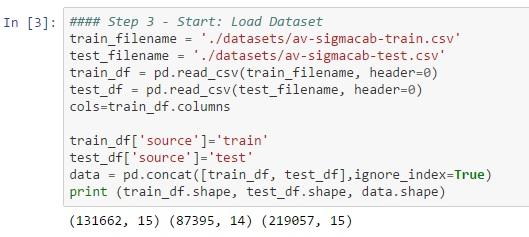
#步骤3 - 加载训练数据集
#步骤4 - 了解数据(描述性统计,可视化)
#步骤5 - 数据预处理(处理缺失数据和异常值,特征工程,特征变换等)
#步骤6 - 功能选择
#步骤7 - 创建验证集
#步骤8 - 比较算法,找到候选算法
#步骤9 - 算法调整
#步骤10 - 完成模型
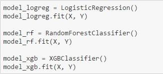
在这种情况下,我们在训练数据上安装了3个模型,以便比较得到的解释。3个模型是a)逻辑回归,b)Random Forest,c)XGBoost。
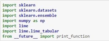
LIME步骤1 - 安装LIME(在ANACONDA分布中 - pip安装LIME)之后,导入相关的库,如下所示:
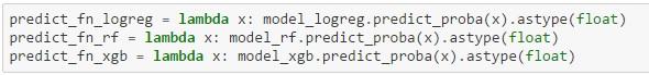
LIME步骤2 - 为每个分类器创建一个lambda函数,该函数将返回给定特征集的目标变量(峰时定价类型)的预测概率
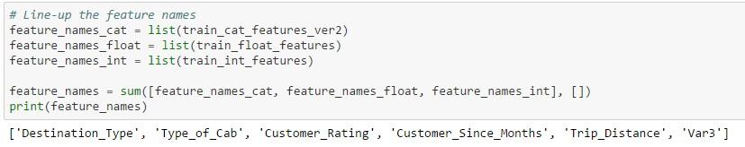
LIME步骤3 - 创建所有功能名称的连接列表,这些列表将在后续步骤中由LIME解释器使用
LIME步骤4 - 这是创建解释器的“神奇”步骤

该函数使用的参数有:
X_train =训练集
feature_names =所有功能名称的连接列表
class_names =目标值
categorical_features =数据集中的分类列的列表
categoriesical_names =分类列名称列表
Kernel width =参数控制诱导模型的线性度,模型的宽度越大,线性越大。
LIME步骤5 - 从LIME获取验证数据集中特定值的说明
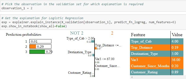
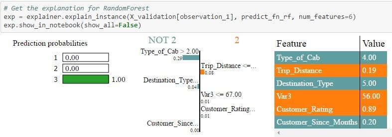
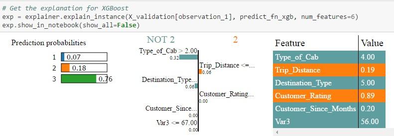
在验证数据集中选择特定观察值,以获得每个类的概率值。LIME将对分配概率的原因进行说明。将概率值与预测目标变量的实际类别进行比较。
输出显示2次观察:
验证集中的Id = 2:所有三种算法都将一个较高的概率赋值为3,这就是实际值。但Random Forest分配最大概率的概率为0.7到1.0。此外,您可以看到不同算法分配给每个功能的权重是完全不同的。另外,当您查看NOT 2 | 2表,您可以看到不同算法对每个功能分配的权重。例如,在逻辑回归的情况下,Cab> 2的类型被分配的权重为0.12,在Random Forest的情况下,权重为0.29,在Xgboost的情况下为0.32。然后将每个特征进行颜色编码,以指示它是否有助于特征值表中的2(橙色)或NOT 2(灰色)的预测。 Feature-Value表本身显示该特定记录的功能的实际值(在这种情况下为Id = 2)
(注意:可视化功能不足以显示多类场景中所有类的功能权重,但同样的过程也适用于区分1类和3类)
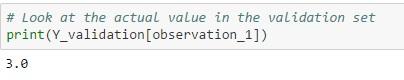
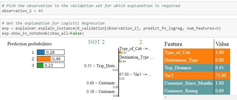
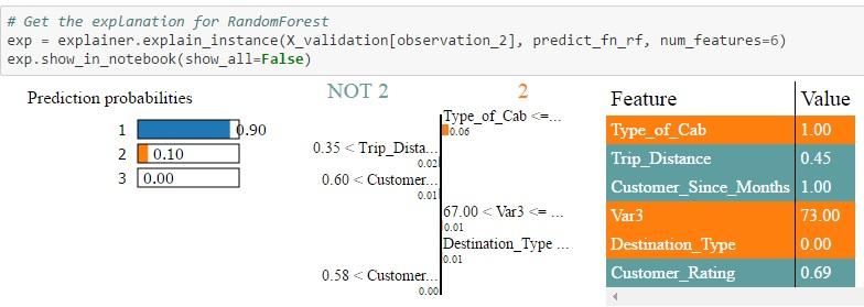
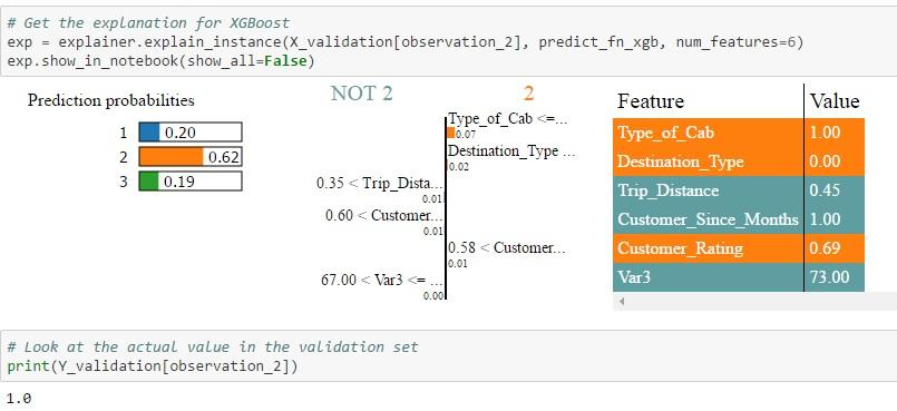
2.验证集中的Id = 45:在这种情况下,只有Random Forest能够为类型1分配更高的概率,也是实际值。逻辑回归和XGBoost都预测2型会有较高的概率。另外,当您查看NOT 2 | 2表,您可以看到不同算法为每个功能分配的权重。例如,在逻辑回归的情况下,行驶距离> 0.35的权重分配为0.01,在Random Forest的情况下为0.02,在Xgboost的情况下为0.01。然后将每个特征进行颜色编码,以指示它是否有助于特征值表中的2(橙色)或NOT 2(灰色)的预测。Feature-Value表本身显示该特定记录的功能的实际值(在这种情况下为Id = 45)
(注意:可视化功能不足以显示多类场景中所有类的功能权重,但同样的过程也适用于区分1类和3类)
每个算法的概率值是不同的,因为每个算法计算的特征权重不同。根据特定记录的特征的实际值和分配给这些特征的权重,用算法计算类的概率,然后预测具有最高概率的类。这些结果可以由主题专家来解释,以查看哪个算法拾取正确的信号/特征以进行预测。本质上,黑盒算法已经成为白盒,现在我们知道是什么驱动算法进行预测。
以下是整个代码供您参考
看到这些结果,我希望您和我一样兴奋。LIME的输出为机器学习算法的内部工作提供了一个直观的预测功能。如果LIME或类似的算法可以帮助黑盒算法提供可解释的输出,那么就从商业用户获取信任。通过建立这种信任,可以在商业环境中进行有效的部署,实现更高准确性和可解释性。请仔细阅读LIME论文,了解它背后的数学。
此文为编译作品,作者Karthikeyan Sankaran ,原网站
https://www.analyticsvidhya.com/blog/2017/06/building-trust-in-machine-learning-models/
约翰·斯特拉
介绍
现在越来越多的公司意识到数据的强大。机器学习模型越来越受欢迎,现在正在使用数据来解决各种商业问题。话虽如此,模型的准确性和可解释性之间总是存在着取舍。
一般来说,如果准确性得到提高,数据科学家必须使用复杂的算法,如Bagging,Boosting,Random Forests等,这些都是“黑盒”的方法。Kaggle或Google Analytics(分析)Vidhya比赛中的许多获奖作品往往会使用像XGBoost这样的算法,不需要向商业用户解释生成预测的过程。另一方面,在商业环境中,更多使用具有说明性的比较简单的模型,如线性回归,逻辑回归,决策树等,即使预测不太准确。
这种情况必须改变 - 准确性和可解释性之间的取舍是不能接受的。我们需要找到使用强大的黑匣算法的方法,即使在商业环境中,仍然能够直观地向用户解释预测背后的逻辑。随着对预测信任的增加,将在企业内更广泛地部署机器学习模型。问题是 - “ 我们如何建立对机器学习模型的信任 ”?
1、动机
正是在这种情况下,我对论文“为什么我相信您” - 解释分类器的预测非常感兴趣。在本文中[1] ,作者解释了一个叫LIME的框架,这是一种算法,可以用一种正确的方式对分类器或回归量的预测进行解释,通过一个可说明的模型来做局部预测。在本文中,有许多问题的例子,其中黑盒算法(即使像深度学习一样极端)的预测可以用可解释的方式来表述。我不会在这个博客中解释这篇文章,而是展示它如何在我们自己的分类问题中实现。
2.问题
Sigma Cab的峰时定价类型分类
今年二月,Analytics Vidhya举办了机器学习比赛,其目标是预测Sigma Cab的“峰时定价类型” - 出租车聚合服务。这是一个多类分类的问题。在这个博客中,我们将看到如何对这个数据集做出预测,并使用LIME来做出预测的解释。这里的意图不是建立最好的模式,而是重点在于可解释性方面。
2.1建模模型的步骤
#步骤1 - 导入所有库
#步骤2 - 定义函数,变量和辞典
#步骤3 - 加载训练数据集
#步骤4 - 了解数据(描述性统计,可视化)
#步骤5 - 数据预处理(处理缺失数据和异常值,特征工程,特征变换等)
#步骤6 - 功能选择
#步骤7 - 创建验证集
#步骤8 - 比较算法,找到候选算法
#步骤9 - 算法调整
#步骤10 - 完成模型
在这种情况下,我们在训练数据上安装了3个模型,以便比较得到的解释。3个模型是a)逻辑回归,b)Random Forest,c)XGBoost。
2.2用Lime使模型可解释的步骤
LIME步骤1 - 安装LIME(在ANACONDA分布中 - pip安装LIME)之后,导入相关的库,如下所示:
LIME步骤2 - 为每个分类器创建一个lambda函数,该函数将返回给定特征集的目标变量(峰时定价类型)的预测概率
LIME步骤3 - 创建所有功能名称的连接列表,这些列表将在后续步骤中由LIME解释器使用
LIME步骤4 - 这是创建解释器的“神奇”步骤
该函数使用的参数有:
X_train =训练集
feature_names =所有功能名称的连接列表
class_names =目标值
categorical_features =数据集中的分类列的列表
categoriesical_names =分类列名称列表
Kernel width =参数控制诱导模型的线性度,模型的宽度越大,线性越大。
LIME步骤5 - 从LIME获取验证数据集中特定值的说明
在验证数据集中选择特定观察值,以获得每个类的概率值。LIME将对分配概率的原因进行说明。将概率值与预测目标变量的实际类别进行比较。
输出显示2次观察:
验证集中的Id = 2:所有三种算法都将一个较高的概率赋值为3,这就是实际值。但Random Forest分配最大概率的概率为0.7到1.0。此外,您可以看到不同算法分配给每个功能的权重是完全不同的。另外,当您查看NOT 2 | 2表,您可以看到不同算法对每个功能分配的权重。例如,在逻辑回归的情况下,Cab> 2的类型被分配的权重为0.12,在Random Forest的情况下,权重为0.29,在Xgboost的情况下为0.32。然后将每个特征进行颜色编码,以指示它是否有助于特征值表中的2(橙色)或NOT 2(灰色)的预测。 Feature-Value表本身显示该特定记录的功能的实际值(在这种情况下为Id = 2)
(注意:可视化功能不足以显示多类场景中所有类的功能权重,但同样的过程也适用于区分1类和3类)
2.验证集中的Id = 45:在这种情况下,只有Random Forest能够为类型1分配更高的概率,也是实际值。逻辑回归和XGBoost都预测2型会有较高的概率。另外,当您查看NOT 2 | 2表,您可以看到不同算法为每个功能分配的权重。例如,在逻辑回归的情况下,行驶距离> 0.35的权重分配为0.01,在Random Forest的情况下为0.02,在Xgboost的情况下为0.01。然后将每个特征进行颜色编码,以指示它是否有助于特征值表中的2(橙色)或NOT 2(灰色)的预测。Feature-Value表本身显示该特定记录的功能的实际值(在这种情况下为Id = 45)
(注意:可视化功能不足以显示多类场景中所有类的功能权重,但同样的过程也适用于区分1类和3类)
每个算法的概率值是不同的,因为每个算法计算的特征权重不同。根据特定记录的特征的实际值和分配给这些特征的权重,用算法计算类的概率,然后预测具有最高概率的类。这些结果可以由主题专家来解释,以查看哪个算法拾取正确的信号/特征以进行预测。本质上,黑盒算法已经成为白盒,现在我们知道是什么驱动算法进行预测。
以下是整个代码供您参考
# Load All Libraries

import pandas as pd

import numpy as np

import matplotlib.pyplot as plt

import seaborn as sns

from sklearn.base import TransformerMixin

from sklearn.preprocessing import Imputer

from sklearn.preprocessing import MinMaxScaler

from sklearn.preprocessing import LabelEncoder

from sklearn.metrics import accuracy_score

from sklearn import cross_validation

from sklearn.linear_model import LogisticRegression

from sklearn.ensemble import RandomForestClassifier

from xgboost import XGBClassifier


#### Write your functions and define variables

def num_missing(x):

  return sum(x.isnull())


class DataFrameImputer(TransformerMixin):


    def __init__(self):

        """Impute missing values.


        Columns of dtype object are imputed with the most frequent value

        in column.


        Columns of other types are imputed with mean of column.


        """

    def fit(self, X, y=None):


        self.fill = pd.Series([X[c].value_counts().index[0]

            if X[c].dtype == np.dtype('O') else X[c].mean() for c in X],

            index=X.columns)


        return self


    def transform(self, X, y=None):

        return X.fillna(self.fill)


#### Load Dataset

train_filename = './datasets/av-sigmacab-train.csv'

test_filename = './datasets/av-sigmacab-test.csv'

train_df = pd.read_csv(train_filename, header=0)

test_df = pd.read_csv(test_filename, header=0)

cols=train_df.columns


train_df['source']='train'

test_df['source']='test'

data = pd.concat([train_df, test_df],ignore_index=True)

print (train_df.shape, test_df.shape, data.shape)


# Handling missing values

imputer_mean = Imputer(missing_values = 'NaN', strategy = 'mean', axis = 0)

imputer_median = Imputer(missing_values = 'NaN', strategy = 'median', axis = 0)

imputer_mode = Imputer(missing_values = 'NaN', strategy = 'most_frequent', axis = 0)


data["Life_Style_Index"]=imputer_mean.fit_transform(data[["Life_Style_Index"]]).ravel()

data["Var1"]=imputer_mean.fit_transform(data[["Var1"]]).ravel()

data["Customer_Since_Months"]=imputer_median.fit_transform(data[["Customer_Since_Months"]]).ravel()


X = pd.DataFrame(data)

data = DataFrameImputer().fit_transform(X)

print (data.apply(num_missing, axis=0))


#Divide into test and train:

train_df = data.loc[data['source']=="train"]

test_df = data.loc[data['source']=="test"]


# Drop unwanted columns

train_df = train_df.drop(['Trip_ID','Cancellation_Last_1Month','Confidence_Life_Style_Index','Gender','Life_Style_Index','Var1','Var2','source',],axis=1)

#### Extract the label column

train_target = np.ravel(np.array(train_df['Surge_Pricing_Type'].values))

train_df = train_df.drop(['Surge_Pricing_Type'],axis=1)


# Extract features

float_columns=[]

cat_columns=[]

int_columns=[]


for i in train_df.columns:

    if train_df[i].dtype == 'float' :

        float_columns.append(i)

    elif train_df[i].dtype == 'int64':

        int_columns.append(i)

    elif train_df[i].dtype == 'object':

        cat_columns.append(i)


train_cat_features = train_df[cat_columns]

train_float_features = train_df[float_columns]

train_int_features = train_df[int_columns]


## Transformation of categorical columns

# Label Encoding:

#train_cat_features_ver2 = pd.get_dummies(train_cat_features, columns=['Destination_Type','Type_of_Cab'])

train_cat_features_ver2 = train_cat_features.apply(LabelEncoder().fit_transform)


## Transformation of float columns

# Rescale data (between 0 and 1)

scaler = MinMaxScaler(feature_range=(0, 1))


for i in train_float_features.columns:

    X_temp = train_float_features[i].reshape(-1,1)

    train_float_features[i] = scaler.fit_transform(X_temp)


#### Finalize X & Y

temp_1 = np.concatenate((train_cat_features_ver2,train_float_features),axis=1)

train_transformed_features = np.concatenate((temp_1,train_int_features),axis=1)

train_transformed_features = pd.DataFrame(data=train_transformed_features)


array = train_transformed_features.values

number_of_features = len(array[0])

X = array[:,0:number_of_features]

Y = train_target


# Split into training and validation set

validation_size = 0.2

seed = 7

X_train, X_validation, Y_train, Y_validation = cross_validation.train_test_split(X, Y, test_size=validation_size, random_state=seed)


scoring = 'accuracy'


# Model 1 - Logisitic Regression

model_logreg = LogisticRegression()

model_logreg.fit(X_train, Y_train)

accuracy_score(Y_validation, model_logreg.predict(X_validation))


# Model 2 - RandomForest Classifier

model_rf = RandomForestClassifier()

model_rf.fit(X_train, Y_train)

accuracy_score(Y_validation, model_rf.predict(X_validation))


# Model 3 - XGB Classifier

model_xgb = XGBClassifier()

model_xgb.fit(X_train, Y_train)

accuracy_score(Y_validation, model_xgb.predict(X_validation))


model_logreg = LogisticRegression()

model_logreg.fit(X, Y)


model_rf = RandomForestClassifier()

model_rf.fit(X, Y)


model_xgb = XGBClassifier()

model_xgb.fit(X, Y)


# LIME SECTION

import sklearn

import sklearn.datasets

import sklearn.ensemble

import numpy as np

import lime

import lime.lime_tabular

from __future__ import print_function


predict_fn_logreg = lambda x: model_logreg.predict_proba(x).astype(float)

predict_fn_rf = lambda x: model_rf.predict_proba(x).astype(float)

predict_fn_xgb = lambda x: model_xgb.predict_proba(x).astype(float)


# Line-up the feature names

feature_names_cat = list(train_cat_features_ver2)

feature_names_float = list(train_float_features)

feature_names_int = list(train_int_features)


feature_names = sum([feature_names_cat, feature_names_float, feature_names_int], [])

print(feature_names)


# Create the LIME Explainer

explainer = lime.lime_tabular.LimeTabularExplainer(X_train ,feature_names = feature_names,class_names=['1','2','3'],

                                                   categorical_features=cat_columns,

                                                   categorical_names=feature_names_cat, kernel_width=3)


# Pick the observation in the validation set for which explanation is required

observation_1 = 2


# Get the explanation for Logistic Regression

exp = explainer.explain_instance(X_validation[observation_1], predict_fn_logreg, num_features=6)

exp.show_in_notebook(show_all=False)


# Get the explanation for RandomForest

exp = explainer.explain_instance(X_validation[observation_1], predict_fn_rf, num_features=6)

exp.show_in_notebook(show_all=False)


# Get the explanation for XGBoost

exp = explainer.explain_instance(X_validation[observation_1], predict_fn_xgb, num_features=6)

exp.show_in_notebook(show_all=False)


# Look at the actual value in the validation set

print(Y_validation[observation_1])


# Pick the observation in the validation set for which explanation is required

observation_2 = 45


# Get the explanation for Logistic Regression

exp = explainer.explain_instance(X_validation[observation_2], predict_fn_logreg, num_features=6)

exp.show_in_notebook(show_all=False)


# Get the explanation for RandomForest

exp = explainer.explain_instance(X_validation[observation_2], predict_fn_rf, num_features=6)

exp.show_in_notebook(show_all=False)


# Get the explanation for XGBoost

exp = explainer.explain_instance(X_validation[observation_2], predict_fn_xgb, num_features=6)

exp.show_in_notebook(show_all=False)


# Look at the actual value in the validation set

print(Y_validation[observation_2])
3.最后
看到这些结果,我希望您和我一样兴奋。LIME的输出为机器学习算法的内部工作提供了一个直观的预测功能。如果LIME或类似的算法可以帮助黑盒算法提供可解释的输出,那么就从商业用户获取信任。通过建立这种信任,可以在商业环境中进行有效的部署,实现更高准确性和可解释性。请仔细阅读LIME论文,了解它背后的数学。
此文为编译作品,作者Karthikeyan Sankaran ,原网站
https://www.analyticsvidhya.com/blog/2017/06/building-trust-in-machine-learning-models/

欢迎关注ATYUN官方公众号
商务合作及内容投稿请联系邮箱:bd@atyun.com


广告


写评论取消
回复取消