


请先登录您的atyun账户,方可使用该功能

审核通过后即可使用此功能,请耐心等待~


Python机器学习的练习八:异常检测和推荐系统
2018年06月01日 由 xiaoshan.xiang 发表
581630
0
Python机器学习的练习系列共有八个部分:
Python机器学习的练习一:简单线性回归
Python机器学习的练习二:多元线性回归
Python机器学习的练习三:逻辑回归
Python机器学习的练习四:多元逻辑回归
Python机器学习的练习五:神经网络
Python机器学习的练习六:支持向量机
Python机器学习的练习七:K-Means聚类和主成分分析
Python机器学习的练习八:异常检测和推荐系统
在Python机器学习的练习八,这篇文章中,将会涉及两个话题——异常检测和推荐系统,我们将使用高斯模型实现异常检测算法并且应用它检测网络上的故障服务器。我们还将看到如何使用协同过滤创建推荐系统,并将其应用于电影推荐数据集。
我们的第一个任务是利用高斯模型判断数据集里未标记的例子是否应该被认为是异常的。我们可以在简单的二维数据集上开始,这样就可以很容易的看到算法如何工作。
加载数据并绘图。
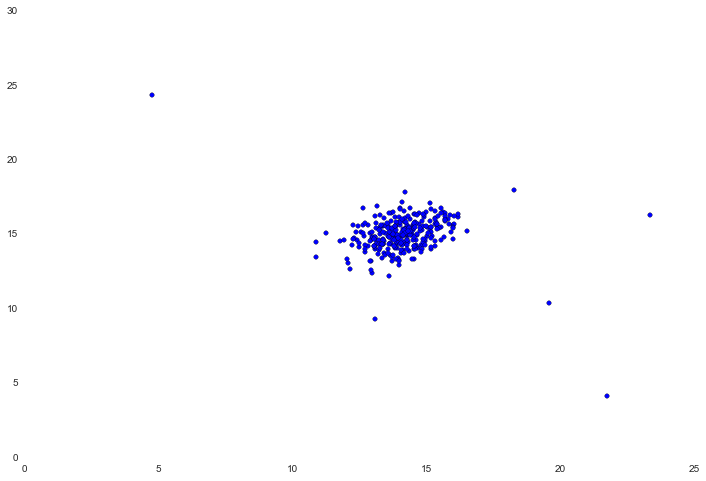
在中心有一个非常紧密的集群,有几个值离集群比较远。在这个简单的例子中,这几个值可以被视为异常。为了找到原因,我们需要估算数据中每个特征的高斯分布。我们需要用均值和方差定义概率分布。为此,我们将创建一个简单的函数,计算数据集中每个特征的均值和方差。
现在我们已经有了模型参数,接下来需要确定概率阈值,它用来表明例子应该是否被视为异常值。我们需要使用一系列标签验证数据(真正的异常数据已经被标出),并且在给出不同阈值的情况下测试模型的识别性能。
我们还需要一种方法来计算数据点属于给定参数集正态分布的概率。幸运的是SciPy内置了这种方法。
在不清楚的情况下,我们只需要计算数据集第一维度的前50个实例的分布概率,这些概率是通过计算该维度的均值和方差得到的。
在我们计算的高斯模型参数中,计算并保存数据集中的每一个值的概率密度。
我们还需要为验证集(使用相同的模型参数)执行此操作。我们将使用这些概率和真实标签来确定最优概率阈值,进而指定数据点作为异常值。
接下来我们需要一个函数,在给出的概率密度和真实标签中找到最佳阈值。为了执行这步操作,我们需要计算不同值的epsilon的F1分数,F1是true positive, false positive和 false negative数值的函数。
最后我们在数据集上应用阈值,可视化结果。
结果还不错,红色的点是被标记为离群值的点,视觉上这些看起来很合理。有一些分离(但没有被标记)的右上角的点也可能是一个离群值,但这是相当接近的。
推荐系统使用项目和基于用户的相似性计算,以检查用户的历史偏好,从而为用户推荐可能感兴趣的新“东西”。在这个练习中,我们将实现一种特殊的推荐算法,称为协同过滤,并将其应用于电影评分的数据集。首先加载并检查我们要处理的数据。
Y是一个包含从一到五的评分的数据组,R是一个包含二进制值的“指示器”数据组,它表明了用户是否对电影进行了评分。两者应该具有相同的形状。
我们可以通过Y中的一行平均值来评估电影的平均评分。
如果它是图片的话,我们也通过渲染矩阵来可视化数据。
接下来我们将实现协同过滤的成本函数。“成本”是指电影评分预测偏离真实预测的程度。在文本练习中,成本函数是给定的。它以文本中的X和Theta参数矩阵为基础,这些展开到参数输入中,以便使用SciPy的优化包。注意,我已经在注释中包含了数组/矩阵形状,以帮助说明矩阵交互如何工作。
我们提供一系列预先训练过并且我们可以评估的参数进行测试。为了减少评估时间,我们研究较小的子集。
答案与练习文本中的结果匹配。接下来需要实现梯度计算,与练习四中神经网络的实现一样,我们会扩展成本函数计算梯度。
下一步是在成本和梯度计算中添加正则化。最终会创建一个正则化版本的函数。(注意,这个版本包含一个额外的学习速率参数“lambda”)
结果与执行代码的预期输出匹配,看起来正则化是有效的。在训练模型之前,还有最后一步:创建我们自己的电影评分模型,这样我们就可以使用这个模型来生成个性化的建议。我们得到了一个将电影索引链接到其标题的文件。把文件加载到字典中,并使用练习文本提供的一些样本评分。
我们可以在数据集中添加自定义评分向量。
开始训练协同过滤模型,我们将通过成本函数、参数向量和输入的数据矩阵使评分正规化,并且运行优化程序。
由于所有的优化程序都是“unrolled”,因此要正确地工作,需要将我们的矩阵重新调整回原来的维度。
我们训练过的参数有X和Theta,使用这些为我们以前添加的用户提供建议。
这给了我们一个有序的最高评分名单,但我们失去了评分的索引。我们需要使用argsort来了解预测评分对应的电影。
实际上推荐的电影并没有很好地符合练习文本中的内容。原因不太清楚,我还没有找到任何可以解释的理由,在代码中可能有错误。不过,即使有一些细微的差别,这个例子的大部分也是准确的。
最后的练习结束了!
Python机器学习的练习一:简单线性回归
Python机器学习的练习二:多元线性回归
Python机器学习的练习三:逻辑回归
Python机器学习的练习四:多元逻辑回归
Python机器学习的练习五:神经网络
Python机器学习的练习六:支持向量机
Python机器学习的练习七:K-Means聚类和主成分分析
Python机器学习的练习八:异常检测和推荐系统
在Python机器学习的练习八,这篇文章中,将会涉及两个话题——异常检测和推荐系统,我们将使用高斯模型实现异常检测算法并且应用它检测网络上的故障服务器。我们还将看到如何使用协同过滤创建推荐系统,并将其应用于电影推荐数据集。
异常检测
我们的第一个任务是利用高斯模型判断数据集里未标记的例子是否应该被认为是异常的。我们可以在简单的二维数据集上开始,这样就可以很容易的看到算法如何工作。
加载数据并绘图。
import numpy as np

import pandas as pd

import matplotlib.pyplot as plt

import seaborn as sb

from scipy.io import loadmat

%matplotlib inline


data = loadmat('data/ex8data1.mat')

X = data['X']

X.shape
(307L, 2L)
fig, ax = plt.subplots(figsize=(12,8))

ax.scatter(X[:,0], X[:,1])
在中心有一个非常紧密的集群,有几个值离集群比较远。在这个简单的例子中,这几个值可以被视为异常。为了找到原因,我们需要估算数据中每个特征的高斯分布。我们需要用均值和方差定义概率分布。为此,我们将创建一个简单的函数,计算数据集中每个特征的均值和方差。
def estimate_gaussian(X):

    mu = X.mean(axis=0)

    sigma = X.var(axis=0)


    return mu, sigma


mu, sigma = estimate_gaussian(X)

mu, sigma
(array([ 14.11222578, 14.99771051]), array([ 1.83263141, 1.70974533]))
现在我们已经有了模型参数,接下来需要确定概率阈值,它用来表明例子应该是否被视为异常值。我们需要使用一系列标签验证数据(真正的异常数据已经被标出),并且在给出不同阈值的情况下测试模型的识别性能。
Xval = data['Xval']

yval = data['yval']


Xval.shape, yval.shape
((307L, 2L), (307L, 1L))
我们还需要一种方法来计算数据点属于给定参数集正态分布的概率。幸运的是SciPy内置了这种方法。
from scipy import stats

dist = stats.norm(mu[0], sigma[0])

dist.pdf(X[:,0])[0:50]
array([ 0.183842  ,  0.20221694,  0.21746136,  0.19778763,  0.20858956,

        0.21652359,  0.16991291,  0.15123542,  0.1163989 ,  0.1594734 ,

        0.21716057,  0.21760472,  0.20141857,  0.20157497,  0.21711385,

        0.21758775,  0.21695576,  0.2138258 ,  0.21057069,  0.1173018 ,

        0.20765108,  0.21717452,  0.19510663,  0.21702152,  0.17429399,

        0.15413455,  0.21000109,  0.20223586,  0.21031898,  0.21313426,

        0.16158946,  0.2170794 ,  0.17825767,  0.17414633,  0.1264951 ,

        0.19723662,  0.14538809,  0.21766361,  0.21191386,  0.21729442,

        0.21238912,  0.18799417,  0.21259798,  0.21752767,  0.20616968,

        0.21520366,  0.1280081 ,  0.21768113,  0.21539967,  0.16913173])
在不清楚的情况下,我们只需要计算数据集第一维度的前50个实例的分布概率,这些概率是通过计算该维度的均值和方差得到的。
在我们计算的高斯模型参数中,计算并保存数据集中的每一个值的概率密度。
p = np.zeros((X.shape[0], X.shape[1]))

p[:,0] = stats.norm(mu[0], sigma[0]).pdf(X[:,0])

p[:,1] = stats.norm(mu[1], sigma[1]).pdf(X[:,1])


p.shape
(307L, 2L)
我们还需要为验证集(使用相同的模型参数)执行此操作。我们将使用这些概率和真实标签来确定最优概率阈值,进而指定数据点作为异常值。
pval = np.zeros((Xval.shape[0], Xval.shape[1]))

pval[:,0] = stats.norm(mu[0], sigma[0]).pdf(Xval[:,0])

pval[:,1] = stats.norm(mu[1], sigma[1]).pdf(Xval[:,1])
接下来我们需要一个函数,在给出的概率密度和真实标签中找到最佳阈值。为了执行这步操作,我们需要计算不同值的epsilon的F1分数,F1是true positive, false positive和 false negative数值的函数。
def select_threshold(pval, yval):

    best_epsilon = 0

    best_f1 = 0

    f1 = 0


    step = (pval.max() - pval.min()) / 1000


    for epsilon in np.arange(pval.min(), pval.max(), step):

        preds = pval < epsilon


        tp = np.sum(np.logical_and(preds == 1, yval == 1)).astype(float)

        fp = np.sum(np.logical_and(preds == 1, yval == 0)).astype(float)

        fn = np.sum(np.logical_and(preds == 0, yval == 1)).astype(float)


        precision = tp / (tp + fp)

        recall = tp / (tp + fn)

        f1 = (2 * precision * recall) / (precision + recall)


        if f1 > best_f1:

            best_f1 = f1

            best_epsilon = epsilon


    return best_epsilon, best_f1


epsilon, f1 = select_threshold(pval, yval)

epsilon, f1
(0.0095667060059568421, 0.7142857142857143)
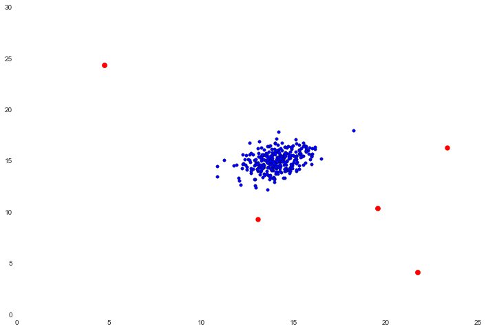
最后我们在数据集上应用阈值,可视化结果。
# indexes of the values considered to be outliers

outliers = np.where(p < epsilon)


fig, ax = plt.subplots(figsize=(12,8))

ax.scatter(X[:,0], X[:,1])

ax.scatter(X[outliers[0],0], X[outliers[0],1], s=50, color='r', marker='o')
结果还不错,红色的点是被标记为离群值的点,视觉上这些看起来很合理。有一些分离(但没有被标记)的右上角的点也可能是一个离群值,但这是相当接近的。
协同过滤
推荐系统使用项目和基于用户的相似性计算,以检查用户的历史偏好,从而为用户推荐可能感兴趣的新“东西”。在这个练习中,我们将实现一种特殊的推荐算法,称为协同过滤,并将其应用于电影评分的数据集。首先加载并检查我们要处理的数据。
data = loadmat('data/ex8_movies.mat')

data
{'R': array([[1, 1, 0, ..., 1, 0, 0],
[1, 0, 0, ..., 0, 0, 1],
[1, 0, 0, ..., 0, 0, 0],
...,
[0, 0, 0, ..., 0, 0, 0],
[0, 0, 0, ..., 0, 0, 0],
[0, 0, 0, ..., 0, 0, 0]], dtype=uint8),
'Y': array([[5, 4, 0, ..., 5, 0, 0],
[3, 0, 0, ..., 0, 0, 5],
[4, 0, 0, ..., 0, 0, 0],
...,
[0, 0, 0, ..., 0, 0, 0],
[0, 0, 0, ..., 0, 0, 0],
[0, 0, 0, ..., 0, 0, 0]], dtype=uint8),
'__globals__': [],
'__header__': 'MATLAB 5.0 MAT-file, Platform: GLNXA64, Created on: Thu Dec 1 17:19:26 2011',
'__version__': '1.0'}Y是一个包含从一到五的评分的数据组,R是一个包含二进制值的“指示器”数据组,它表明了用户是否对电影进行了评分。两者应该具有相同的形状。
Y = data['Y']

R = data['R']

Y.shape, R.shape
((1682L, 943L), (1682L, 943L))
我们可以通过Y中的一行平均值来评估电影的平均评分。
Y[1,R[1,:]].mean()
2.5832449628844114
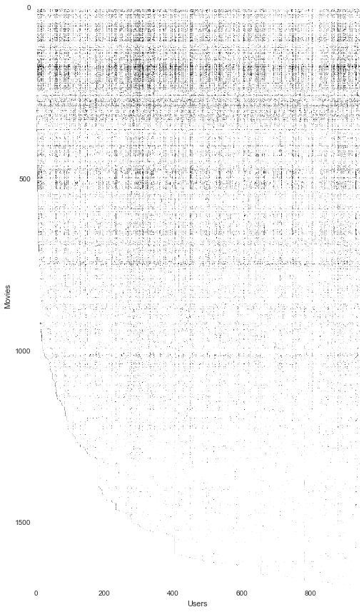
如果它是图片的话,我们也通过渲染矩阵来可视化数据。
fig, ax = plt.subplots(figsize=(12,12))

ax.imshow(Y)

ax.set_xlabel('Users')

ax.set_ylabel('Movies')

fig.tight_layout()
接下来我们将实现协同过滤的成本函数。“成本”是指电影评分预测偏离真实预测的程度。在文本练习中,成本函数是给定的。它以文本中的X和Theta参数矩阵为基础,这些展开到参数输入中,以便使用SciPy的优化包。注意,我已经在注释中包含了数组/矩阵形状,以帮助说明矩阵交互如何工作。
def cost(params, Y, R, num_features):

    Y = np.matrix(Y)  # (1682, 943)

    R = np.matrix(R)  # (1682, 943)

    num_movies = Y.shape[0]

    num_users = Y.shape[1]


    # reshape the parameter array into parameter matrices

    X = np.matrix(np.reshape(params[:num_movies * num_features], (num_movies, num_features)))  # (1682, 10)

    Theta = np.matrix(np.reshape(params[num_movies * num_features:], (num_users, num_features)))  # (943, 10)


    # initializations

    J = 0


    # compute the cost

    error = np.multiply((X * Theta.T) - Y, R)  # (1682, 943)

    squared_error = np.power(error, 2)  # (1682, 943)

    J = (1. / 2) * np.sum(squared_error)


    return J
我们提供一系列预先训练过并且我们可以评估的参数进行测试。为了减少评估时间,我们研究较小的子集。
users = 4

movies = 5

features = 3


params_data = loadmat('data/ex8_movieParams.mat')

X = params_data['X']

Theta = params_data['Theta']


X_sub = X[:movies, :features]

Theta_sub = Theta[:users, :features]

Y_sub = Y[:movies, :users]

R_sub = R[:movies, :users]


params = np.concatenate((np.ravel(X_sub), np.ravel(Theta_sub)))


cost(params, Y_sub, R_sub, features)
22.224603725685675
答案与练习文本中的结果匹配。接下来需要实现梯度计算,与练习四中神经网络的实现一样,我们会扩展成本函数计算梯度。
def cost(params, Y, R, num_features):

    Y = np.matrix(Y)  # (1682, 943)

    R = np.matrix(R)  # (1682, 943)

    num_movies = Y.shape[0]

    num_users = Y.shape[1]


    # reshape the parameter array into parameter matrices

    X = np.matrix(np.reshape(params[:num_movies * num_features], (num_movies, num_features)))  # (1682, 10)

    Theta = np.matrix(np.reshape(params[num_movies * num_features:], (num_users, num_features)))  # (943, 10)


    # initializations

    J = 0

    X_grad = np.zeros(X.shape)  # (1682, 10)

    Theta_grad = np.zeros(Theta.shape)  # (943, 10)


    # compute the cost

    error = np.multiply((X * Theta.T) - Y, R)  # (1682, 943)

    squared_error = np.power(error, 2)  # (1682, 943)

    J = (1. / 2) * np.sum(squared_error)


    # calculate the gradients

    X_grad = error * Theta

    Theta_grad = error.T * X


    # unravel the gradient matrices into a single array

    grad = np.concatenate((np.ravel(X_grad), np.ravel(Theta_grad)))


    return J, grad


J, grad = cost(params, Y_sub, R_sub, features)

J, grad
(22.224603725685675,

 array([ -2.52899165,   7.57570308,  -1.89979026,  -0.56819597,

          3.35265031,  -0.52339845,  -0.83240713,   4.91163297,

         -0.76677878,  -0.38358278,   2.26333698,  -0.35334048,

         -0.80378006,   4.74271842,  -0.74040871, -10.5680202 ,

          4.62776019,  -7.16004443,  -3.05099006,   1.16441367,

         -3.47410789,   0.        ,   0.        ,   0.        ,

          0.        ,   0.        ,   0.        ]))
下一步是在成本和梯度计算中添加正则化。最终会创建一个正则化版本的函数。(注意,这个版本包含一个额外的学习速率参数“lambda”)
def cost(params, Y, R, num_features, learning_rate):

    Y = np.matrix(Y)  # (1682, 943)

    R = np.matrix(R)  # (1682, 943)

    num_movies = Y.shape[0]

    num_users = Y.shape[1]


    # reshape the parameter array into parameter matrices

    X = np.matrix(np.reshape(params[:num_movies * num_features], (num_movies, num_features)))  # (1682, 10)

    Theta = np.matrix(np.reshape(params[num_movies * num_features:], (num_users, num_features)))  # (943, 10)


    # initializations

    J = 0

    X_grad = np.zeros(X.shape)  # (1682, 10)

    Theta_grad = np.zeros(Theta.shape)  # (943, 10)


    # compute the cost

    error = np.multiply((X * Theta.T) - Y, R)  # (1682, 943)

    squared_error = np.power(error, 2)  # (1682, 943)

    J = (1. / 2) * np.sum(squared_error)


    # add the cost regularization

    J = J + ((learning_rate / 2) * np.sum(np.power(Theta, 2)))

    J = J + ((learning_rate / 2) * np.sum(np.power(X, 2)))


    # calculate the gradients with regularization

    X_grad = (error * Theta) + (learning_rate * X)

    Theta_grad = (error.T * X) + (learning_rate * Theta)


    # unravel the gradient matrices into a single array

    grad = np.concatenate((np.ravel(X_grad), np.ravel(Theta_grad)))


    return J, grad


J, grad = cost(params, Y_sub, R_sub, features, 1.5)

J, grad
(31.344056244274221,

 array([ -0.95596339,   6.97535514,  -0.10861109,   0.60308088,

          2.77421145,   0.25839822,   0.12985616,   4.0898522 ,

         -0.89247334,   0.29684395,   1.06300933,   0.66738144,

          0.60252677,   4.90185327,  -0.19747928, -10.13985478,

          2.10136256,  -6.76563628,  -2.29347024,   0.48244098,

         -2.99791422,  -0.64787484,  -0.71820673,   1.27006666,

          1.09289758,  -0.40784086,   0.49026541]))
结果与执行代码的预期输出匹配,看起来正则化是有效的。在训练模型之前,还有最后一步:创建我们自己的电影评分模型,这样我们就可以使用这个模型来生成个性化的建议。我们得到了一个将电影索引链接到其标题的文件。把文件加载到字典中,并使用练习文本提供的一些样本评分。
movie_idx = {}

f = open('data/movie_ids.txt')

for line in f:

    tokens = line.split(' ')

    tokens[-1] = tokens[-1][:-1]

    movie_idx[int(tokens[0]) - 1] = ' '.join(tokens[1:])


ratings = np.zeros((1682, 1))


ratings[0] = 4

ratings[6] = 3

ratings[11] = 5

ratings[53] = 4

ratings[63] = 5

ratings[65] = 3

ratings[68] = 5

ratings[97] = 2

ratings[182] = 4

ratings[225] = 5

ratings[354] = 5


print('Rated {0} with {1} stars.'.format(movie_idx[0], str(int(ratings[0]))))

print('Rated {0} with {1} stars.'.format(movie_idx[6], str(int(ratings[6]))))

print('Rated {0} with {1} stars.'.format(movie_idx[11], str(int(ratings[11]))))

print('Rated {0} with {1} stars.'.format(movie_idx[53], str(int(ratings[53]))))

print('Rated {0} with {1} stars.'.format(movie_idx[63], str(int(ratings[63]))))

print('Rated {0} with {1} stars.'.format(movie_idx[65], str(int(ratings[65]))))

print('Rated {0} with {1} stars.'.format(movie_idx[68], str(int(ratings[68]))))

print('Rated {0} with {1} stars.'.format(movie_idx[97], str(int(ratings[97]))))

print('Rated {0} with {1} stars.'.format(movie_idx[182], str(int(ratings[182]))))

print('Rated {0} with {1} stars.'.format(movie_idx[225], str(int(ratings[225]))))

print('Rated {0} with {1} stars.'.format(movie_idx[354], str(int(ratings[354]))))
Rated Toy Story (1995) with 4 stars.
Rated Twelve Monkeys (1995) with 3 stars.
Rated Usual Suspects, The (1995) with 5 stars.
Rated Outbreak (1995) with 4 stars.
Rated Shawshank Redemption, The (1994) with 5 stars.
Rated While You Were Sleeping (1995) with 3 stars.
Rated Forrest Gump (1994) with 5 stars.
Rated Silence of the Lambs, The (1991) with 2 stars.
Rated Alien (1979) with 4 stars.
Rated Die Hard 2 (1990) with 5 stars.
Rated Sphere (1998) with 5 stars.
我们可以在数据集中添加自定义评分向量。
R = data['R']

Y = data['Y']


Y = np.append(Y, ratings, axis=1)

R = np.append(R, ratings != 0, axis=1)
开始训练协同过滤模型,我们将通过成本函数、参数向量和输入的数据矩阵使评分正规化,并且运行优化程序。
from scipy.optimize import minimize


movies = Y.shape[0]

users = Y.shape[1]

features = 10

learning_rate = 10.


X = np.random.random(size=(movies, features))

Theta = np.random.random(size=(users, features))

params = np.concatenate((np.ravel(X), np.ravel(Theta)))


Ymean = np.zeros((movies, 1))

Ynorm = np.zeros((movies, users))


for i in range(movies):

    idx = np.where(R[i,:] == 1)[0]

    Ymean[i] = Y[i,idx].mean()

    Ynorm[i,idx] = Y[i,idx] - Ymean[i]


fmin = minimize(fun=cost, x0=params, args=(Ynorm, R, features, learning_rate),

                method='CG', jac=True, options={'maxiter': 100})

fmin
   status: 1

 success: False

    njev: 149

    nfev: 149

     fun: 38953.88249706676

       x: array([-0.07177334, -0.08315075,  0.1081135 , ...,  0.1817828 ,

        0.16873062,  0.03383596])

 message: 'Maximum number of iterations has been exceeded.'

     jac: array([ 0.01833555,  0.07377974,  0.03999323, ..., -0.00970181,

        0.00758961, -0.01181811])
由于所有的优化程序都是“unrolled”,因此要正确地工作,需要将我们的矩阵重新调整回原来的维度。
X = np.matrix(np.reshape(fmin.x[:movies * features], (movies, features)))

Theta = np.matrix(np.reshape(fmin.x[movies * features:], (users, features)))


X.shape, Theta.shape
((1682L, 10L), (944L, 10L))
我们训练过的参数有X和Theta,使用这些为我们以前添加的用户提供建议。
predictions = X * Theta.T

my_preds = predictions[:, -1] + Ymean

sorted_preds = np.sort(my_preds, axis=0)[::-1]

sorted_preds[:10]
matrix([[ 5.00000264],

        [ 5.00000249],

        [ 4.99999831],

        [ 4.99999671],

        [ 4.99999659],

        [ 4.99999253],

        [ 4.99999238],

        [ 4.9999915 ],

        [ 4.99999019],

        [ 4.99998643]]
这给了我们一个有序的最高评分名单,但我们失去了评分的索引。我们需要使用argsort来了解预测评分对应的电影。
idx = np.argsort(my_preds, axis=0)[::-1]

print("Top 10 movie predictions:")

for i in range(10):

    j = int(idx[i])

    print('Predicted rating of {0} for movie {1}.'.format(str(float(my_preds[j])), movie_idx[j]))
Top 10 movie predictions:

Predicted rating of 5.00000264002 for movie Prefontaine (1997).

Predicted rating of 5.00000249142 for movie Santa with Muscles (1996).

Predicted rating of 4.99999831018 for movie Marlene Dietrich: Shadow and Light (1996) .

Predicted rating of 4.9999967124 for movie Saint of Fort Washington, The (1993).

Predicted rating of 4.99999658864 for movie They Made Me a Criminal (1939).

Predicted rating of 4.999992533 for movie Someone Else's America (1995).

Predicted rating of 4.99999238336 for movie Great Day in Harlem, A (1994).

Predicted rating of 4.99999149604 for movie Star Kid (1997).

Predicted rating of 4.99999018592 for movie Aiqing wansui (1994).

Predicted rating of 4.99998642746 for movie Entertaining Angels: The Dorothy Day Story (1996).
实际上推荐的电影并没有很好地符合练习文本中的内容。原因不太清楚,我还没有找到任何可以解释的理由,在代码中可能有错误。不过,即使有一些细微的差别,这个例子的大部分也是准确的。
最后的练习结束了!

欢迎关注ATYUN官方公众号
商务合作及内容投稿请联系邮箱:bd@atyun.com


广告


广告

写评论取消
回复取消