


请先登录您的atyun账户,方可使用该功能

审核通过后即可使用此功能,请耐心等待~


Python机器学习的练习七:K-Means聚类和主成分分析
2018年06月01日 由 xiaoshan.xiang 发表
530468
0
Python机器学习的练习系列共有八个部分:
Python机器学习的练习一:简单线性回归
Python机器学习的练习二:多元线性回归
Python机器学习的练习三:逻辑回归
Python机器学习的练习四:多元逻辑回归
Python机器学习的练习五:神经网络
Python机器学习的练习六:支持向量机
Python机器学习的练习七:K-Means聚类和主成分分析
Python机器学习的练习八:异常检测和推荐系统
Python机器学习的练习七,涵盖两个吸引人的话题:K-Means聚类和主成分分析(PCA),K-Means和PCA都是无监督学习技术的例子,无监督学习问题没有为我们提供任何标签或者目标去学习做出预测,所以无监督算法试图从数据本身中学习一些有趣的结构,我们将首先实现k-means,并了解如何使用它来压缩图像。我们还将用PCA进行实验,以发现面部图像的低维度表示。
首先,我们在一个简单的二维数据集上实现并应用k-means,以了解它如何工作。k-means是一种迭代的、无监督的聚类算法,它将类似的实例组合成集群。该算法通过猜测每个集群的初始centroid,反复向最近的集群分配实例,并重新计算该集群的centroid。首先我们要实现一个函数,它为数据中的每个实例找到最接近的centroid。
测试函数确保它像预期的那样工作,我们使用练习中的测试案例。
输出与文本中的预期值相匹配(我们的数组是zero-indexed而不是one-indexed,所以值比练习中的值要低1)。接下来,我们需要一个函数来计算集群的centroid。centroid是当前分配给集群的所有例子的平均值。
此输出也与该练习的预期值相匹配。目前为止一切都很顺利。下一部分涉及到实际运行算法的迭代次数和可视化结果。我们在练习中实现了这一步骤,它没有那么复杂,我将从头开始构建它。为了运行这个算法,我们只需要在分配到最近集群的示例和重新计算集群的centroids之间进行交替操作。
我们现在可以使用颜色编码表示集群成员。
我们跳过了初始化centroid的过程。这可能会影响算法的收敛性。
接下来创建一个可以选择随机例子的函数,并将这些例子作为初始的centroid。
我们的下一任务是应用K-means实现图像压缩。我们可以使用集群来查找图像中最具有代表性的少量的颜色,并使用集群分配将原来的24位颜色映射到一个低维度的颜色空间。这是我们要压缩的图像。
原始像素数据已经预加载了,把它输入进来。
我们可以快速查看数据的形状,以验证它是否像我们预期的图像。
现在我们需要对数据进行预处理,并将它输入到k-means算法中。
我们在压缩中创建了一些artifact,尽管将原始图像映射到仅16种颜色,但图像的主要特征仍然存在。
这是关于k-means的部分,接下来我们来看关于主成分分析的部分。
PCA是一个可以在数据集中找到“主成分”或者最大方差方向的线性变换。它可以用于其他事物的维度减少。在这个练习中,我们需要实现PCA,并将其应用于一个简单的二维数据集,观察它是如何工作的。从加载和可视化数据集开始。
PCA的算法相当简单。在保证数据正规化后,输出只是原始数据协方差矩阵的单值分解。由于numpy已经有内置函数来计算矩阵协方差和SVD,我们将利用这些函数而不是从头开始。
现在我们已经有了主成分(矩阵U),我们可以利用它把原始数据投入到一个更低维度的空间,对于这个任务,我们将实现一个函数,它计算投影并只选择顶部K成分,有效地减少了维度的数量。
我们也可以通过改变采取的步骤来恢复原始数据。
如果我们尝试去可视化恢复的数据,会很容易的发现算法的工作原理。
注意这些点如何被压缩成一条虚线。虚线本质上是第一个主成分。当我们将数据减少到一个维度时,我们切断的第二个主成分可以被认为是与这条虚线的正交变化。由于我们失去了这些信息,我们的重建只能将这些点与第一个主成分相关联。
我们这次练习的最后一项任务是将PCA应用于脸部图像。通过使用相同降维技术,我们可以使用比原始图像少得多的数据来捕捉图像的“本质”。
该练习代码包含一个函数,它将在网格中的数据集中渲染前100个脸部图像。你可以在练习文本中找到它们,不需要重新生成。
只有32 x 32灰度图像。下一步我们要在脸部图像数据集上运行PCA,并取得前100个主成分。
现在尝试恢复原来的结构并重新渲染它。
结果并没有像预期的维度数量减少10倍,可能是因为我们丢失了一些细节部分。
Python机器学习的练习一:简单线性回归
Python机器学习的练习二:多元线性回归
Python机器学习的练习三:逻辑回归
Python机器学习的练习四:多元逻辑回归
Python机器学习的练习五:神经网络
Python机器学习的练习六:支持向量机
Python机器学习的练习七:K-Means聚类和主成分分析
Python机器学习的练习八:异常检测和推荐系统
Python机器学习的练习七,涵盖两个吸引人的话题:K-Means聚类和主成分分析(PCA),K-Means和PCA都是无监督学习技术的例子,无监督学习问题没有为我们提供任何标签或者目标去学习做出预测,所以无监督算法试图从数据本身中学习一些有趣的结构,我们将首先实现k-means,并了解如何使用它来压缩图像。我们还将用PCA进行实验,以发现面部图像的低维度表示。
K-Means聚类
首先,我们在一个简单的二维数据集上实现并应用k-means,以了解它如何工作。k-means是一种迭代的、无监督的聚类算法,它将类似的实例组合成集群。该算法通过猜测每个集群的初始centroid,反复向最近的集群分配实例,并重新计算该集群的centroid。首先我们要实现一个函数,它为数据中的每个实例找到最接近的centroid。
import numpy as np

import pandas as pd

import matplotlib.pyplot as plt

import seaborn as sb

from scipy.io import loadmat

%matplotlib inline


def find_closest_centroids(X, centroids):

    m = X.shape[0]

    k = centroids.shape[0]

    idx = np.zeros(m)


    for i in range(m):

        min_dist = 1000000

        for j in range(k):

            dist = np.sum((X[i,:] - centroids[j,:]) ** 2)

            if dist < min_dist:

                min_dist = dist

                idx[i] = j


    return idx
测试函数确保它像预期的那样工作,我们使用练习中的测试案例。
data = loadmat('data/ex7data2.mat')

X = data['X']

initial_centroids = initial_centroids = np.array([[3, 3], [6, 2], [8, 5]])


idx = find_closest_centroids(X, initial_centroids)

idx[0:3]
array([ 0., 2., 1.])
输出与文本中的预期值相匹配(我们的数组是zero-indexed而不是one-indexed,所以值比练习中的值要低1)。接下来,我们需要一个函数来计算集群的centroid。centroid是当前分配给集群的所有例子的平均值。
def compute_centroids(X, idx, k):

    m, n = X.shape

    centroids = np.zeros((k, n))


    for i in range(k):

        indices = np.where(idx == i)

        centroids[i,:] = (np.sum(X[indices,:], axis=1) / len(indices[0])).ravel()


    return centroids


compute_centroids(X, idx, 3)
array([[ 2.42830111,  3.15792418],

       [ 5.81350331,  2.63365645],

       [ 7.11938687,  3.6166844 ]])
此输出也与该练习的预期值相匹配。目前为止一切都很顺利。下一部分涉及到实际运行算法的迭代次数和可视化结果。我们在练习中实现了这一步骤,它没有那么复杂,我将从头开始构建它。为了运行这个算法,我们只需要在分配到最近集群的示例和重新计算集群的centroids之间进行交替操作。
def run_k_means(X, initial_centroids, max_iters):

    m, n = X.shape

    k = initial_centroids.shape[0]

    idx = np.zeros(m)

    centroids = initial_centroids


    for i in range(max_iters):

        idx = find_closest_centroids(X, centroids)

        centroids = compute_centroids(X, idx, k)


    return idx, centroids


idx, centroids = run_k_means(X, initial_centroids, 10)
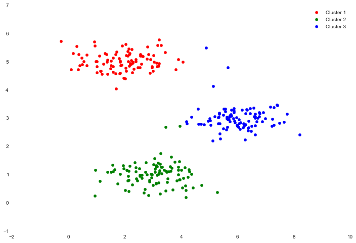
我们现在可以使用颜色编码表示集群成员。
cluster1 = X[np.where(idx == 0)[0],:]

cluster2 = X[np.where(idx == 1)[0],:]

cluster3 = X[np.where(idx == 2)[0],:]


fig, ax = plt.subplots(figsize=(12,8))

ax.scatter(cluster1[:,0], cluster1[:,1], s=30, color='r', label='Cluster 1')

ax.scatter(cluster2[:,0], cluster2[:,1], s=30, color='g', label='Cluster 2')

ax.scatter(cluster3[:,0], cluster3[:,1], s=30, color='b', label='Cluster 3')

ax.legend()
我们跳过了初始化centroid的过程。这可能会影响算法的收敛性。
接下来创建一个可以选择随机例子的函数,并将这些例子作为初始的centroid。
def init_centroids(X, k):

    m, n = X.shape

    centroids = np.zeros((k, n))

    idx = np.random.randint(0, m, k)


    for i in range(k):

        centroids[i,:] = X[idx[i],:]


    return centroids


init_centroids(X, 3)
array([[ 1.15354031,  4.67866717],

       [ 6.27376271,  2.24256036],

       [ 2.20960296,  4.91469264]])
我们的下一任务是应用K-means实现图像压缩。我们可以使用集群来查找图像中最具有代表性的少量的颜色,并使用集群分配将原来的24位颜色映射到一个低维度的颜色空间。这是我们要压缩的图像。
原始像素数据已经预加载了,把它输入进来。
image_data = loadmat('data/bird_small.mat')

image_data
{'A': array([[[219, 180, 103],
[230, 185, 116],
[226, 186, 110],
...,
[ 14, 15, 13],
[ 13, 15, 12],
[ 12, 14, 12]],
...,
[[ 15, 19, 19],
[ 20, 20, 18],
[ 18, 19, 17],
...,
[ 65, 43, 39],
[ 58, 37, 38],
[ 52, 39, 34]]], dtype=uint8),
'__globals__': [],
'__header__': 'MATLAB 5.0 MAT-file, Platform: GLNXA64, Created on: Tue Jun 5 04:06:24 2012',
'__version__': '1.0'}我们可以快速查看数据的形状,以验证它是否像我们预期的图像。
A = image_data['A']

A.shape
(128L, 128L, 3L)
现在我们需要对数据进行预处理,并将它输入到k-means算法中。
# normalize value ranges
A = A / 255.
# reshape the array
X = np.reshape(A, (A.shape[0] * A.shape[1], A.shape[2]))
# randomly initialize the centroids
initial_centroids = init_centroids(X, 16)
# run the algorithm
idx, centroids = run_k_means(X, initial_centroids, 10)
# get the closest centroids one last time
idx = find_closest_centroids(X, centroids)
# map each pixel to the centroid value
X_recovered = centroids[idx.astype(int),:]
# reshape to the original dimensions
X_recovered = np.reshape(X_recovered, (A.shape[0], A.shape[1], A.shape[2]))
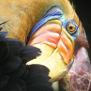
plt.imshow(X_recovered)
我们在压缩中创建了一些artifact,尽管将原始图像映射到仅16种颜色,但图像的主要特征仍然存在。
这是关于k-means的部分,接下来我们来看关于主成分分析的部分。
主成分分析
PCA是一个可以在数据集中找到“主成分”或者最大方差方向的线性变换。它可以用于其他事物的维度减少。在这个练习中,我们需要实现PCA,并将其应用于一个简单的二维数据集,观察它是如何工作的。从加载和可视化数据集开始。
data = loadmat('data/ex7data1.mat')

X = data['X']


fig, ax = plt.subplots(figsize=(12,8))

ax.scatter(X[:, 0], X[:, 1])
PCA的算法相当简单。在保证数据正规化后,输出只是原始数据协方差矩阵的单值分解。由于numpy已经有内置函数来计算矩阵协方差和SVD,我们将利用这些函数而不是从头开始。
def pca(X):

    # normalize the features

    X = (X - X.mean()) / X.std()


    # compute the covariance matrix

    X = np.matrix(X)

    cov = (X.T * X) / X.shape[0]


    # perform SVD

    U, S, V = np.linalg.svd(cov)


    return U, S, V


U, S, V = pca(X)

U, S, V
(matrix([[-0.79241747, -0.60997914],

         [-0.60997914,  0.79241747]]),

 array([ 1.43584536,  0.56415464]),

 matrix([[-0.79241747, -0.60997914],

         [-0.60997914,  0.79241747]]))
现在我们已经有了主成分(矩阵U),我们可以利用它把原始数据投入到一个更低维度的空间,对于这个任务,我们将实现一个函数,它计算投影并只选择顶部K成分,有效地减少了维度的数量。
def project_data(X, U, k):

    U_reduced = U[:,:k]

    return np.dot(X, U_reduced)


Z = project_data(X, U, 1)

Z
matrix([[-4.74689738],

        [-7.15889408],

        [-4.79563345],

        [-4.45754509],

        [-4.80263579],

        ...,

        [-6.44590096],

        [-2.69118076],

        [-4.61386195],

        [-5.88236227],

        [-7.76732508]])
我们也可以通过改变采取的步骤来恢复原始数据。
def recover_data(Z, U, k):

    U_reduced = U[:,:k]

    return np.dot(Z, U_reduced.T)


X_recovered = recover_data(Z, U, 1)

X_recovered
matrix([[ 3.76152442,  2.89550838],

        [ 5.67283275,  4.36677606],

        [ 3.80014373,  2.92523637],

        [ 3.53223661,  2.71900952],

        [ 3.80569251,  2.92950765],

        ...,

        [ 5.10784454,  3.93186513],

        [ 2.13253865,  1.64156413],

        [ 3.65610482,  2.81435955],

        [ 4.66128664,  3.58811828],

        [ 6.1549641 ,  4.73790627]])
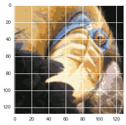
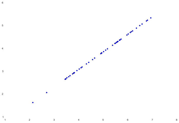
如果我们尝试去可视化恢复的数据,会很容易的发现算法的工作原理。
fig, ax = plt.subplots(figsize=(12,8))

ax.scatter(X_recovered[:, 0], X_recovered[:, 1])
注意这些点如何被压缩成一条虚线。虚线本质上是第一个主成分。当我们将数据减少到一个维度时,我们切断的第二个主成分可以被认为是与这条虚线的正交变化。由于我们失去了这些信息,我们的重建只能将这些点与第一个主成分相关联。
我们这次练习的最后一项任务是将PCA应用于脸部图像。通过使用相同降维技术,我们可以使用比原始图像少得多的数据来捕捉图像的“本质”。
faces = loadmat('data/ex7faces.mat')

X = faces['X']

X.shape
(5000L, 1024L)
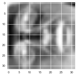
该练习代码包含一个函数,它将在网格中的数据集中渲染前100个脸部图像。你可以在练习文本中找到它们,不需要重新生成。
face = np.reshape(X[3,:], (32, 32))

plt.imshow(face)
只有32 x 32灰度图像。下一步我们要在脸部图像数据集上运行PCA,并取得前100个主成分。
U, S, V = pca(X)

Z = project_data(X, U, 100)
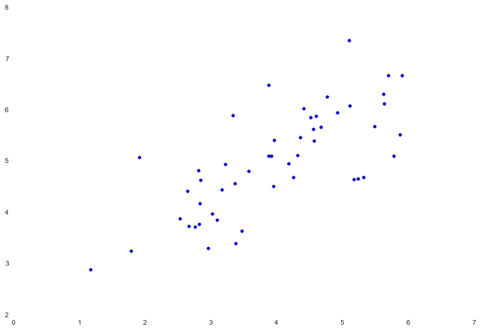
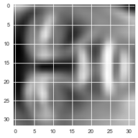
现在尝试恢复原来的结构并重新渲染它。
X_recovered = recover_data(Z, U, 100)

face = np.reshape(X_recovered[3,:], (32, 32))

plt.imshow(face)
结果并没有像预期的维度数量减少10倍,可能是因为我们丢失了一些细节部分。

欢迎关注ATYUN官方公众号
商务合作及内容投稿请联系邮箱:bd@atyun.com


广告


广告

写评论取消
回复取消