


请先登录您的atyun账户,方可使用该功能

审核通过后即可使用此功能,请耐心等待~


深度学习要点:可视化卷积神经网络CNN
2018年03月27日 由 yuxiangyu 发表
393380
0
在本文中,我们将探索如何将卷积神经网络(CNN)可视化。
深度学习中最深入讨论的话题之一是如何解释和理解一个训练完成的模型,尤其是在医疗保健等高风险行业的背景下。“黑盒”这个词经常与深度学习算法联系在一起。如果我们不能解释它是如何工作的,我们如何相信模型的结果呢?
我们将了解卷积神经网络CNN模型可视化的重要性以及将可视化的方法。我们还将研究一个可以帮助您更好地理解概念的实例示例
以一个为了检测癌症肿瘤而训练的深度学习模型为例。该模型告诉你它99%确定它检测到了癌症,但它并没有告诉你为什么或怎么确定的。
它是在MRI扫描(磁共振)中找到了一条重要线索,还是仅仅是扫描中的一个污点被错误地检测为肿瘤?这对患者来说是生死攸关的问题,医生经不起犯错。

正如我们在上面的癌症肿瘤示例中看到的那样,我们了解模型正在做什么以及它是如何做出预测,绝对是至关重要的。通常,下面列出的原因是深度学习实践者要记住的重点:
一般来说,可视化卷积神经网络CNN模型的方法可以根据其工作原理分为三种:
我们会在下面的小节中详细介绍它们。在这里,我们将使用keras作为我们的库,用于构建深度学习卷积神经网络CNN模型,并使用keras-vis来可视化它们。
数据集:https://datahack.analyticsvidhya.com/contest/practice-problem-identify-the-digits/
在开始以下步骤前,确定你已经安装好必要的库,并执行:
我们可以做的最简单的事情就是是打印或者说绘制模型。在这里,你可以打印单层神经网络的形状和每个层的参数。
在keras中,你可以实现它如下:
为了更具创造性和表现力 - 你也可以绘可视化卷积神经网络CNN制架构图(keras.utils.vis_utils函数)。
另一种方法是绘制训练模型的滤波器,以便我们可以了解这些过滤器的行为。例如,上述可视化卷积神经网络CNN模型的第一层的第一个过滤器如下所示:

一般来说,我们可以看到低级滤波器用作边缘检测器,而高级的倾向于捕捉像物品和面部这样的高级概念。
要查看我们的神经网络正在做什么,我们可以在输入图像上应用滤波器,然后绘制输出。这使我们能够理解什么样的输入模式可以激活特定的过滤器。例如,可能会有一个面部过滤器,在图像中出现脸时激活。
我们可以将这个想法转移到所有的类中,并检查每个类的样子。
运行下面的脚本来检查它。
在可视化卷积神经网络CNN图像分类问题中,一个自然的问题是模型是否真的识别出图像中对象的位置,或者只是使用了周边环境。基于遮挡的方法试图通过用灰色方块,系统地遮挡输入图像的不同部分,并监视分类器的输出来回答这个问题。这些例子清楚地显示了模型是在场景中定位对象,因为当物体被遮挡时,正确分类的概率显著下降。
为了理解这个概念,让我们从我们的数据集中取一个随机图像,并尝试绘制图像的热图(heatmap)。这可以让我们直观地看出图像的哪些部分对于该模型最重要,以便对实际的类进行明确的区分。
为了能够了解我们的可视化卷积神经网络CNN模型关注哪个部分来进行预测,我们可以使用特征图。
使用特征图的概念非常简单 - 我们计算对于输入图像的输出分类的梯度。这会告诉我们,输出类别值的改变与输入图像中像素的微小变动之间的联系。梯度中的所有正值都告诉我们,对该像素小的改动会增加输出分类的值。因此,可视化这些与图像形状相同的梯度,应该能提供一些注意力的直觉。
直观地说,这种方法凸显了对输出贡献最大的显著的图像区域。
类激活地图(Class activation maps),即grad-CAM,是对卷积神经网络CNN模型在预测时观察到什么的另一种可视化方法。grad-CAM使用倒数第二个卷积层的输出,而不是使用与输出相关的梯度。这是为了利用存储在倒数第二层中的空间信息。
在本文中,我们介绍了如何可视化卷积神经网络CNN模型,以及为什么要以一个示例来做。希望这会给你一个直觉,告诉你如何在自己的深度学习应用中建立更好的卷积神经网络模型。
深度学习中最深入讨论的话题之一是如何解释和理解一个训练完成的模型,尤其是在医疗保健等高风险行业的背景下。“黑盒”这个词经常与深度学习算法联系在一起。如果我们不能解释它是如何工作的,我们如何相信模型的结果呢?
我们将了解卷积神经网络CNN模型可视化的重要性以及将可视化的方法。我们还将研究一个可以帮助您更好地理解概念的实例示例
以一个为了检测癌症肿瘤而训练的深度学习模型为例。该模型告诉你它99%确定它检测到了癌症,但它并没有告诉你为什么或怎么确定的。
它是在MRI扫描(磁共振)中找到了一条重要线索,还是仅仅是扫描中的一个污点被错误地检测为肿瘤?这对患者来说是生死攸关的问题,医生经不起犯错。
可视化卷积神经网络CNN模型的重要性
正如我们在上面的癌症肿瘤示例中看到的那样,我们了解模型正在做什么以及它是如何做出预测,绝对是至关重要的。通常,下面列出的原因是深度学习实践者要记住的重点:
- 了解模型如何工作
- 协助超参数调优
- 找出模型的失败,并获得他们为什么失败的直觉
- 向消费者/最终用户或业务主管解释决策
可视化卷积神经网络CNN模型的方法
一般来说,可视化卷积神经网络CNN模型的方法可以根据其工作原理分为三种:
- 初步方法 - 简单的展示一个训练完成的可视化卷积神经网络CNN模型的整体结构。
- 基于激活的方法 - 在这种方法中,我们破译单个神经元或一组神经元的激活,以了解他们在做什么的直觉。
- 基于梯度的方法 - 这些方法倾向于在训练可视化卷积神经网络CNN模型时操纵前向和反向传递形成的梯度。
我们会在下面的小节中详细介绍它们。在这里,我们将使用keras作为我们的库,用于构建深度学习卷积神经网络CNN模型,并使用keras-vis来可视化它们。
数据集:https://datahack.analyticsvidhya.com/contest/practice-problem-identify-the-digits/
在开始以下步骤前,确定你已经安装好必要的库,并执行:
%pylab inline

import os

import numpy as np

import pandas as pd

from scipy.misc import imread

from sklearn.metrics import accuracy_score


import keras

from keras.models import Sequential, Model

from keras.layers import Dense, Dropout, Flatten, Activation, Input

from keras.layers import Conv2D, MaxPooling2D


# To stop potential randomness

seed = 128

rng = np.random.RandomState(seed)


data_dir = "../../datasets/MNIST"


train = pd.read_csv('../../datasets/MNIST/train.csv')

test = pd.read_csv('../../datasets/MNIST/Test_fCbTej3.csv')


img_name = rng.choice(train.filename)

filepath = os.path.join(data_dir, 'train', img_name)


img = imread(filepath, flatten=True)


pylab.imshow(img, cmap='gray')

pylab.axis('off')

pylab.show()


temp = []

for img_name in train['filename']:

    image_path = os.path.join(data_dir, 'train', img_name)

    img = imread(image_path, flatten=True)

    img = img.astype('float32')

    temp.append(img)


train_x = np.stack(temp)


train_x /= 255.0

train_x = train_x.reshape(-1, 28, 28, 1).astype('float32')


temp = []

for img_name in test['filename']:

    image_path = os.path.join(data_dir, 'test', img_name)

    img = imread(image_path, flatten=True)

    img = img.astype('float32')

    temp.append(img)


test_x = np.stack(temp)


test_x /= 255.0

test_x = test_x.reshape(-1, 28, 28, 1).astype('float32')


train_y = keras.utils.np_utils.to_categorical(train.label.values)


split_size = int(train_x.shape[0]*0.7)


train_x, val_x = train_x[:split_size], train_x[split_size:]

train_y, val_y = train_y[:split_size], train_y[split_size:]


# define vars


epochs = 5

batch_size = 128


# import keras modules


from keras.models import Sequential

from keras.layers import Dense


# create model

model = Sequential()

model.add(Conv2D(32, kernel_size=(3, 3),

                 activation='relu',

                 input_shape=(28,28, 1)))

model.add(Conv2D(64, (3, 3), activation='relu'))

model.add(MaxPooling2D(pool_size=(2, 2)))

model.add(Dropout(0.25))

model.add(Flatten())

model.add(Dense(128, activation='relu'))

model.add(Dropout(0.5))

model.add(Dense(10, activation='softmax', name='preds'))


# compile the model with necessary attributes

model.compile(loss='categorical_crossentropy', optimizer='adam', metrics=['accuracy'])


trained_model = model.fit(train_x, train_y, nb_epoch=epochs, batch_size=batch_size, validation_data=(val_x, val_y))


pred = model.predict_classes(test_x)


img_name = rng.choice(test.filename)

filepath = os.path.join(data_dir, 'test', img_name)


img = imread(filepath, flatten=True)


test_index = int(img_name.split('.')[0]) - train.shape[0]


print ("Prediction is: ", pred[test_index])


pylab.imshow(img, cmap='gray')

pylab.axis('off')

pylab.show()
1.初步方法
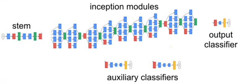
1.1绘制可视化卷积神经网络CNN模型架构
我们可以做的最简单的事情就是是打印或者说绘制模型。在这里,你可以打印单层神经网络的形状和每个层的参数。
在keras中,你可以实现它如下:
model.summary()
_________________________________________________________________

Layer (type)                 Output Shape              Param #

=================================================================

conv2d_1 (Conv2D)            (None, 26, 26, 32)        320

_________________________________________________________________

conv2d_2 (Conv2D)            (None, 24, 24, 64)        18496

_________________________________________________________________

max_pooling2d_1 (MaxPooling2 (None, 12, 12, 64)        0

_________________________________________________________________

dropout_1 (Dropout)          (None, 12, 12, 64)        0

_________________________________________________________________

flatten_1 (Flatten)          (None, 9216)              0

_________________________________________________________________

dense_1 (Dense)              (None, 128)               1179776

_________________________________________________________________

dropout_2 (Dropout)          (None, 128)               0

_________________________________________________________________

preds (Dense)                (None, 10)                1290

=================================================================

Total params: 1,199,882

Trainable params: 1,199,882

Non-trainable params: 0
为了更具创造性和表现力 - 你也可以绘可视化卷积神经网络CNN制架构图(keras.utils.vis_utils函数)。
1.2可视化过滤器
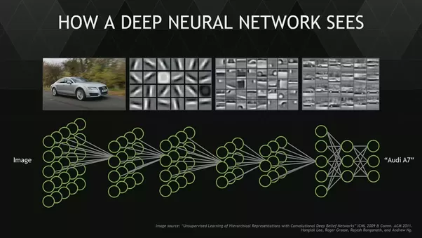
另一种方法是绘制训练模型的滤波器,以便我们可以了解这些过滤器的行为。例如,上述可视化卷积神经网络CNN模型的第一层的第一个过滤器如下所示:
top_layer = model.layers [0]

plt.imshow(top_layer.get_weights()[0] [:,:,:,0] .squeeze(),cmap ='gray')
一般来说,我们可以看到低级滤波器用作边缘检测器,而高级的倾向于捕捉像物品和面部这样的高级概念。
2.激活映射
2.1最大激活
要查看我们的神经网络正在做什么,我们可以在输入图像上应用滤波器,然后绘制输出。这使我们能够理解什么样的输入模式可以激活特定的过滤器。例如,可能会有一个面部过滤器,在图像中出现脸时激活。
from vis.visualization import visualize_activation

from vis.utils import utils

from keras import activations


from matplotlib import pyplot as plt

%matplotlib inline

plt.rcParams['figure.figsize'] = (18, 6)


# Utility to search for layer index by name.

# Alternatively we can specify this as -1 since it corresponds to the last layer.

layer_idx = utils.find_layer_idx(model, 'preds')


# Swap softmax with linear

model.layers[layer_idx].activation = activations.linear

model = utils.apply_modifications(model)


# This is the output node we want to maximize.

filter_idx = 0

img = visualize_activation(model, layer_idx, filter_indices=filter_idx)

plt.imshow(img[..., 0])
我们可以将这个想法转移到所有的类中,并检查每个类的样子。
运行下面的脚本来检查它。
for output_idx in np.arange(10):

   # Lets turn off verbose output this time to avoid clutter and just see the output.

   img = visualize_activation(model, layer_idx, filter_indices=output_idx, input_range=(0., 1.))

   plt.figure()

   plt.title('Networks perception of {}'.format(output_idx))

   plt.imshow(img[..., 0])
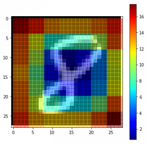
2.2图像遮挡
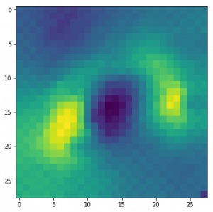
在可视化卷积神经网络CNN图像分类问题中,一个自然的问题是模型是否真的识别出图像中对象的位置,或者只是使用了周边环境。基于遮挡的方法试图通过用灰色方块,系统地遮挡输入图像的不同部分,并监视分类器的输出来回答这个问题。这些例子清楚地显示了模型是在场景中定位对象,因为当物体被遮挡时,正确分类的概率显著下降。
为了理解这个概念,让我们从我们的数据集中取一个随机图像,并尝试绘制图像的热图(heatmap)。这可以让我们直观地看出图像的哪些部分对于该模型最重要,以便对实际的类进行明确的区分。
def iter_occlusion(image, size=8):

    # taken from https://www.kaggle.com/blargl/simple-occlusion-and-saliency-maps


   occlusion = np.full((size * 5, size * 5, 1), [0.5], np.float32)

   occlusion_center = np.full((size, size, 1), [0.5], np.float32)

   occlusion_padding = size * 2


   # print('padding...')

   image_padded = np.pad(image, ( \

   (occlusion_padding, occlusion_padding), (occlusion_padding, occlusion_padding), (0, 0) \

   ), 'constant', constant_values = 0.0)


   for y in range(occlusion_padding, image.shape[0] + occlusion_padding, size):


       for x in range(occlusion_padding, image.shape[1] + occlusion_padding, size):

           tmp = image_padded.copy()


           tmp[y - occlusion_padding:y + occlusion_center.shape[0] + occlusion_padding, \

             x - occlusion_padding:x + occlusion_center.shape[1] + occlusion_padding] \

             = occlusion


           tmp[y:y + occlusion_center.shape[0], x:x + occlusion_center.shape[1]] = occlusion_center


           yield x - occlusion_padding, y - occlusion_padding, \

             tmp[occlusion_padding:tmp.shape[0] - occlusion_padding, occlusion_padding:tmp.shape[1] - occlusion_padding]


i = 23 # for example

data = val_x[i]

correct_class = np.argmax(val_y[i])


# input tensor for model.predict

inp = data.reshape(1, 28, 28, 1)


# image data for matplotlib's imshow

img = data.reshape(28, 28)


# occlusion

img_size = img.shape[0]

occlusion_size = 4


print('occluding...')


heatmap = np.zeros((img_size, img_size), np.float32)

class_pixels = np.zeros((img_size, img_size), np.int16)


from collections import defaultdict

counters = defaultdict(int)


for n, (x, y, img_float) in enumerate(iter_occlusion(data, size=occlusion_size)):


    X = img_float.reshape(1, 28, 28, 1)

    out = model.predict(X)

    #print('#{}: {} @ {} (correct class: {})'.format(n, np.argmax(out), np.amax(out), out[0][correct_class]))

    #print('x {} - {} | y {} - {}'.format(x, x + occlusion_size, y, y + occlusion_size))


    heatmap[y:y + occlusion_size, x:x + occlusion_size] = out[0][correct_class]

    class_pixels[y:y + occlusion_size, x:x + occlusion_size] = np.argmax(out)

    counters[np.argmax(out)] += 1
3.基于梯度的方法
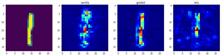
3.1特征图
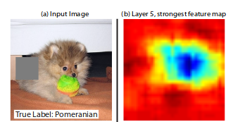
为了能够了解我们的可视化卷积神经网络CNN模型关注哪个部分来进行预测,我们可以使用特征图。
使用特征图的概念非常简单 - 我们计算对于输入图像的输出分类的梯度。这会告诉我们,输出类别值的改变与输入图像中像素的微小变动之间的联系。梯度中的所有正值都告诉我们,对该像素小的改动会增加输出分类的值。因此,可视化这些与图像形状相同的梯度,应该能提供一些注意力的直觉。
直观地说,这种方法凸显了对输出贡献最大的显著的图像区域。
class_idx = 0

indices = np.where(val_y[:, class_idx] == 1.)[0]


# pick some random input from here.

idx = indices[0]


# Lets sanity check the picked image.

from matplotlib import pyplot as plt

%matplotlib inline

plt.rcParams['figure.figsize'] = (18, 6)


plt.imshow(val_x[idx][..., 0])


from vis.visualization import visualize_saliency

from vis.utils import utils

from keras import activations


# Utility to search for layer index by name.

# Alternatively we can specify this as -1 since it corresponds to the last layer.

layer_idx = utils.find_layer_idx(model, 'preds')


# Swap softmax with linear

model.layers[layer_idx].activation = activations.linear

model = utils.apply_modifications(model)


grads = visualize_saliency(model, layer_idx, filter_indices=class_idx, seed_input=val_x[idx])

# Plot with 'jet' colormap to visualize as a heatmap.

plt.imshow(grads, cmap='jet')


# This corresponds to the Dense linear layer.

for class_idx in np.arange(10):

    indices = np.where(val_y[:, class_idx] == 1.)[0]

    idx = indices[0]


    f, ax = plt.subplots(1, 4)

    ax[0].imshow(val_x[idx][..., 0])


    for i, modifier in enumerate([None, 'guided', 'relu']):

        grads = visualize_saliency(model, layer_idx, filter_indices=class_idx,

        seed_input=val_x[idx], backprop_modifier=modifier)

        if modifier is None:

            modifier = 'vanilla'

        ax[i+1].set_title(modifier)

        ax[i+1].imshow(grads, cmap='jet')
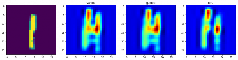
3.2基于梯度的grad-CAM
类激活地图(Class activation maps),即grad-CAM,是对卷积神经网络CNN模型在预测时观察到什么的另一种可视化方法。grad-CAM使用倒数第二个卷积层的输出,而不是使用与输出相关的梯度。这是为了利用存储在倒数第二层中的空间信息。
from vis.visualization import visualize_cam


# This corresponds to the Dense linear layer.

for class_idx in np.arange(10):

 indices = np.where(val_y[:, class_idx] == 1.)[0]

 idx = indices[0]


f, ax = plt.subplots(1, 4)

 ax[0].imshow(val_x[idx][..., 0])


for i, modifier in enumerate([None, 'guided', 'relu']):

    grads = visualize_cam(model, layer_idx, filter_indices=class_idx,

    seed_input=val_x[idx], backprop_modifier=modifier)

    if modifier is None:

        modifier = 'vanilla'

    ax[i+1].set_title(modifier)

    ax[i+1].imshow(grads, cmap='jet')
结语
在本文中,我们介绍了如何可视化卷积神经网络CNN模型,以及为什么要以一个示例来做。希望这会给你一个直觉,告诉你如何在自己的深度学习应用中建立更好的卷积神经网络模型。

欢迎关注ATYUN官方公众号
商务合作及内容投稿请联系邮箱:bd@atyun.com


广告


写评论取消
回复取消